Spectrotemporal processing differences between auditory cortical fast-spiking and regular-spiking neurons

Abstract

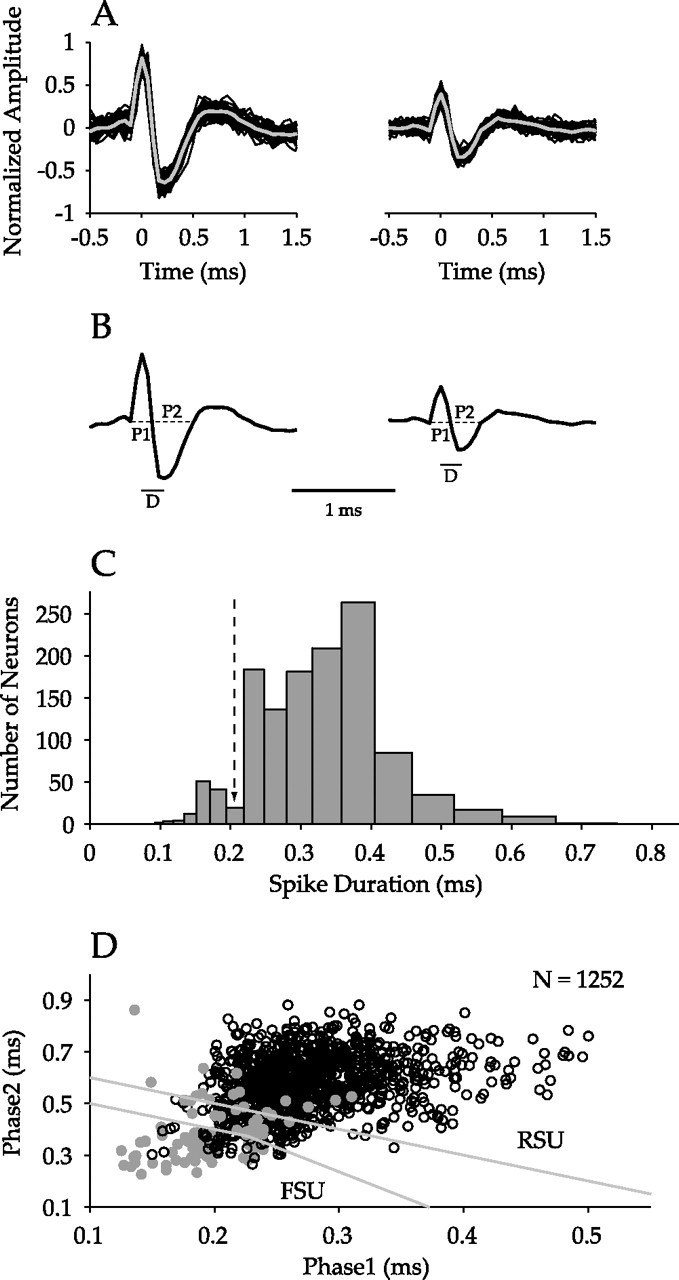
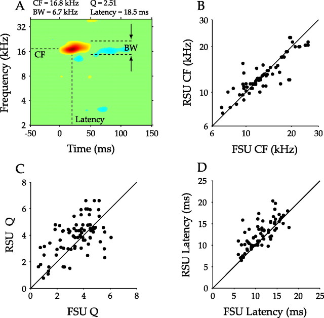
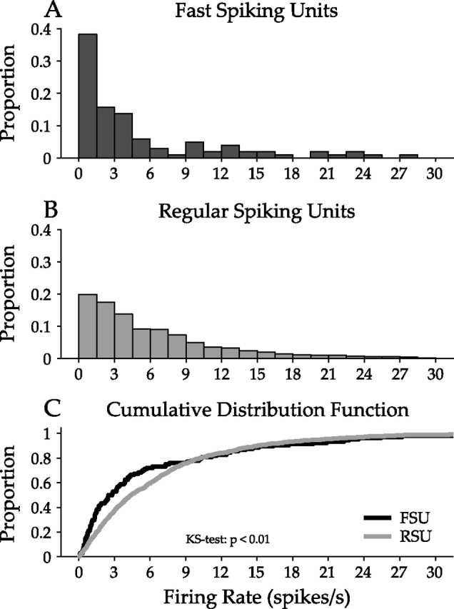
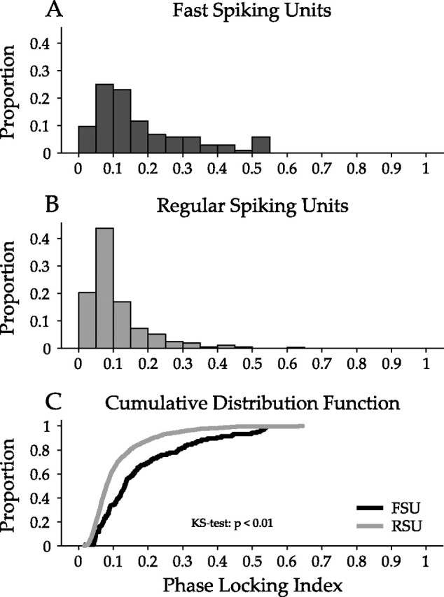
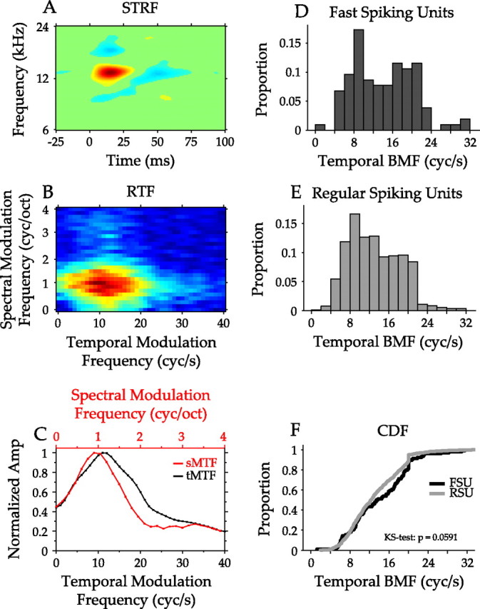
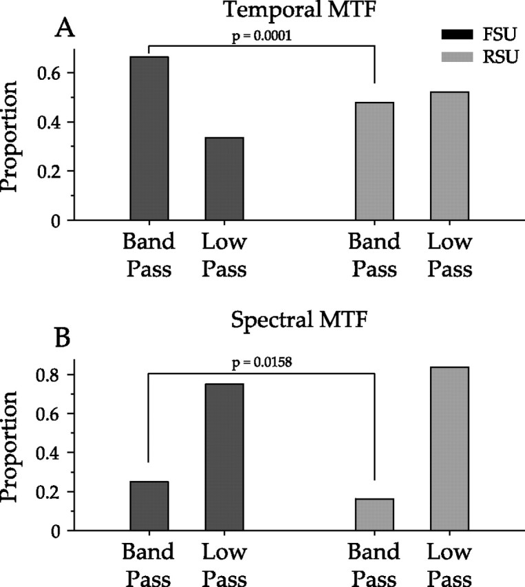
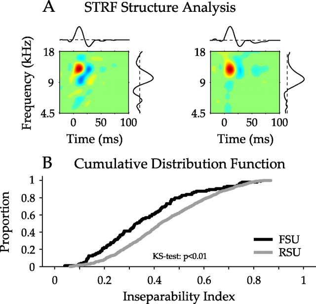
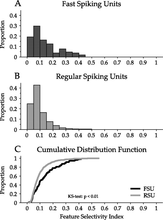
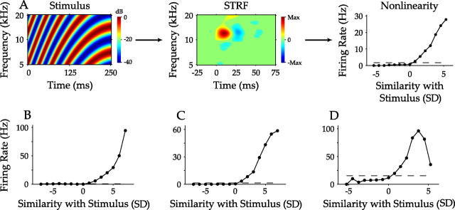
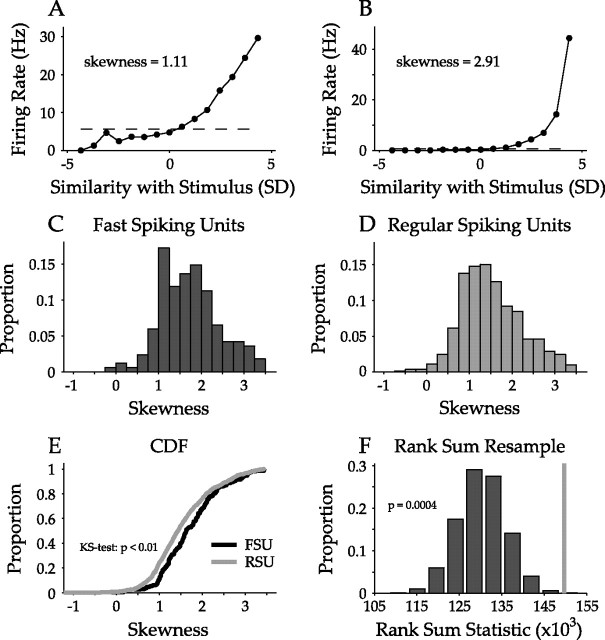
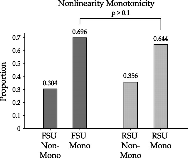
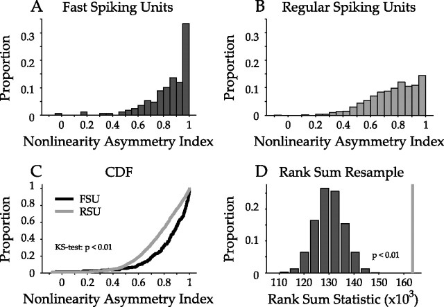
Excitatory pyramidal neurons and inhibitory interneurons constitute the main elements of cortical circuitry and have distinctive morphologic and electrophysiological properties. Here, we differentiate them by analyzing the time course of their action potentials (APs) and characterizing their receptive field properties in auditory cortex. Pyramidal neurons have longer APs and discharge as regular-spiking units (RSUs), whereas basket and chandelier cells, which are inhibitory interneurons, have shorter APs and are fast-spiking units (FSUs). To compare these neuronal classes, we stimulated cat primary auditory cortex neurons with a dynamic moving ripple stimulus and constructed single-unit spectrotemporal receptive fields (STRFs) and their associated nonlinearities. FSUs had shorter latencies, broader spectral tuning, greater stimulus specificity, and higher temporal precision than RSUs. The STRF structure of FSUs was more separable, suggesting more independence between spectral and temporal processing regimens. The nonlinearities associated with the two cell classes were indicative of higher feature selectivity for FSUs. These global functional differences between RSUs and FSUs suggest fundamental distinctions between putative excitatory and inhibitory interneurons that shape auditory cortical processing.

Figure 1.

Classification of AI neurons. A, Two single neurons recorded from the same channel of the multichannel probe. Shown are 50 representative traces (black), with the derived action potential waveform template superimposed (gray). B, Analysis of action potential shape. P1 and P2 denote phase 1 and phase 2, the durations of the two segments of the waveform. D represents the time between the peak and the trough in the waveform. C, Histogram of time between peak and trough in the waveform across all neurons (n = 1252). The dashed arrow at ∼0.2 ms represents the FSU/RSU classification boundary from the study by Mitchell et al. (2007). D, Separation of FSUs and RSUs following the study by Bruno and Simons (2002). By plotting phase 2 against phase 1, FSUs (n = 115) are classified as those neurons falling below the lower gray lines. RSUs (n = 978) are signified by points above the top gray line. Filled gray circles represent neurons for which D ≤ 0.2 ms.

Figure 2.

Depth distribution of recorded AI neurons. A, Distribution of recording depths for FSUs. The abscissa indicates recording position below the cortical surface, whereas the ordinate describes the proportion of the recorded FSU population (n = 115). Two peaks are present from 800–1200 and 1400–1600 μm. B, Distribution of RSUs (n = 978). C, Depth distribution for the ratio of the number of identified FSUs to RSUs. Two FSU peaks are present, as well as an additional peak at 0–200 μm.

Figure 3.

Basic receptive field parameter analysis. A, Parameters obtained from STRFs. The STRF is the average stimulus preceding a spike, with the abscissa representing time before a spike and frequency on the ordinate. Red indicates time–frequency combinations that lead to an increase in firing rate, whereas blue represents a decrease. STRFs are scaled relative to their maximum value. From each STRF, CF, bandwidth (BW), Q values (Q = CF/BW), and the latency were obtained. B, Comparison of FSU and RSU CFs. FSUs and RSUs in the same penetration shared similar CFs. The diagonal line represents equality between the FSU and RSU values. C, Comparison of FSU and RSU sharpness of tuning. Q values were lower for FSUs, indicating that they are more broadly tuned than RSUs. D, Comparison of latencies. FSU latencies were shorter than those of RSUs.

Figure 4.

Comparison of firing rate for FSUs and RSUs. Firing rate was calculated from the response to one dynamic moving ripple stimulus presentation. A, FSU firing rate distribution. The highest proportion of FSUs have firing rates below 6 sp/s. B, The RSU firing rate distribution is approximately exponential, with the proportion of RSUs decaying from low to high firing rates. C, Cumulative distribution functions for FSU and RSU firing rates. The two distributions are significantly different, with FSUs having lower firing rates than RSUs (p < 0.01, KS test).

Figure 5.

Analysis of the temporal precision of FSU and RSU responses. Comparison of phase locking to the ripple stimulus envelope for FSUs and RSUs. The phase-locking index quantifies how well the response is locked to specific temporal aspects of the ripple stimulus. Phase-locking values near 1 indicate precise temporal precision in the response, whereas those near 0 indicate little precision. A, FSU phase-locking distribution extends to 0.55. B, RSU phase-locking distribution extends to 0.3. C, Comparison of phase-locking cumulative distribution functions for FSUs and RSUs. FSUs responded with significantly better temporal precision than RSUs (p < 0.01, KS test).

Figure 6.

Analysis of modulation processing by FSUs and RSUs. A, STRF of a representative AI neuron. The abscissa represents time before a spike. The ordinate represents frequency. Suppression flanks the main excitatory component along the spectral and temporal axes. B, RTF of the STRF in A. The RTF describes the temporal and spectral modulation preferences of an AI neuron and is obtained through the 2D FFT of the STRF. The peak in the RTF is located at ∼10 cycles/s and 1 cycle/octave. C, Temporal and spectral modulation transfer functions obtained from the RTF. The temporal MTF (black) is obtained by summing the RTF across all spectral modulation frequencies. The spectral MTF (red) is obtained by summing across temporal modulation frequencies. The structure of the suppression in the STRF leads to the bandpass structure of the MTFs. D, Temporal best modulation frequency distribution for FSUs. The distribution is relatively uniform from 4 to 22 cycles/s. E, Temporal best modulation frequency distribution for RSUs. F, Comparison of the cumulative distribution functions for temporal best modulation frequency. The FSU and RSU distributions were not significantly different (p = 0.0591, KS test). The distributions for spectral best modulation frequency were also not significantly different (data not shown; p > 0.1, KS test).

Figure 7.

Analysis of modulation transfer function shapes for FSUs and RSUs. Temporal and spectral MTFs were classified as bandpass or low pass (see Materials and Methods). A resampling procedure was then used to determine whether the proportion of bandpass FSUs was significantly different from that of RSUs. Top, Temporal MTF shapes for FSUs and RSUs. A significantly greater proportion of FSUs (65%) compared with RSUs (47%) have bandpass tMTFs (p < 0.01). Bottom, A significantly larger proportion of FSU sMTFs (25%) were bandpass compared with RSUs (15%; p = 0.016).

Figure 8.

Analysis of FSU and RSU STRF structure. For each FSU or RSU, the structure of the STRF was quantified by determining the inseparability of each STRF. A, STRF inseparability analysis for two STRFs. The pair of independent one-dimensional functions that best approximates each STRF is shown. The procedure determines how time and frequency in the STRF may be dissociated. The left STRF is more inseparable (inseparability index of 0.22) than the right STRF (inseparability index of 0.15). B, Inseparability index cumulative distribution functions for FSU and RSU STRFs. Abscissa values near 0 represent STRFs that may be represented by one pair of one-dimensional functions, whereas values near 1 indicate that multiple pairs are required. The receptive fields of FSUs are significantly more separable than those of RSUs (p < 0.01, KS test).

Figure 9.

Analysis of feature selectivity of FSUs and RSUs. The FSI describes the stimulus specificity of a neuron. FSI values near 1 represent a neuron that is selective for only one stimulus feature, whereas values near 0 represent a neuron that is relatively unselective for specific spectrotemporal stimulus patterns. A, Distribution of feature selectivity indices for FSUs. The distribution extends to 0.45, representing moderately strong feature selectivity. B, The FSI distribution for RSUs. C, Comparison of FSI cumulative distribution functions. The FSU distribution is significantly shifted to higher FSIs values, indicating that FSUs are more selective for spectrotemporal stimulus features than RSUs (p < 0.01, KS test).

Figure 10.

Spectrotemporal processing model of auditory cortex neurons. A, The processing of AI neurons may be formulated in three steps: the dynamic moving ripple stimulus is processed by the STRF, the similarity, or correlation, between the STRF and the stimulus is determined, and the result is fed to a nonlinearity; and the nonlinearity determines the firing rate of the neuron as a function of the similarity between the stimulus and STRF. The units of the abscissa, in SDs, represent the likelihood of the stimulus–STRF similarity relative to that expected by a random stimulus. Thus, values near 5 represent stimuli that would be unlikely to be encountered by chance and expected from stimuli that lead to a spike response. B–D, Nonlinearities for three other neurons, displaying strongly monotonic, moderately monotonic, and nonmonotonic behavior. Dashed lines in nonlinearities represent the average firing rate of the neuron.

Figure 11.

Skewness of nonlinearities. A, B, Two nonlinearities with different degrees of skewness. A, When the firing rate slowly increases with stimulus similarity the skewness is ∼1. B, When the rising portion of the nonlinearity is shifted to higher similarity values, the skewness increases to ∼3. C, D, Skewness distributions of FSU and RSU nonlinearities. FSU nonlinearities are shifted to more positive skewness values relative to RSUs. E, Cumulative distribution functions of FSU and RSU nonlinearity skewness values. The FSU distribution is significantly shifted to higher values (p < 0.01, KS test). F, Rank sum analysis of FSU/RSU skewness distributions. The rank sum statistic from the actual data were calculated (gray bar). Then, the FSU and RSU data were combined and resampled with respect to the number of FSUs and RSUs. From the resampled distributions the rank sum statistic was calculated. This process was repeated 10,000 times, and the histogram shows the distribution of these statistics, revealing significance (p = 0.0004).

Figure 12.

Monotonicity of nonlinearities. Monotonicity was determined by first finding the maximum value in each nonlinearity, along with the following two nonlinearity values that corresponded to even higher stimulus similarity values. If the two values that followed the maximum were both less than the maximum value, then the nonlinearity was classified as nonmonotonic (Non-Mono). All other nonlinearities were classified as monotonic (Mono). A total of 69.6% of FSU and 64.4% of RSU nonlinearities were monotonic. Resampling the FSU and RSU distributions revealed that the difference in the proportion of monotonic nonlinearities between of FSUs and RSUs nonlinearities was not significant (p > 0.1).

Figure 13.

Asymmetry of nonlinearities. The asymmetry index of each nonlinearity, which ranges from −1 to +1, was calculated by subtracting the sum of the nonlinearity values for negative STRF similarity values from those for positive values and dividing by the sum of the two. A, B, Distribution of FSU and RSU asymmetry index values. FSUs have a greater proportion of neurons with high asymmetry index values. C, Cumulative distribution functions of asymmetry index values. The FSU distribution is significantly shifted to higher values (p < 0.01, KS test). D, Rank sum analysis of asymmetry index values. The observed rank sum statistic (gray line) is significantly shifted from the resampled distribution (p < 0.01; n = 10,000), further indicating that FSU nonlinearities are more asymmetric than those for RSUs.

References

1. Aertsen A, Johannesma PI. Spectro-temporal receptive fields of auditory neurons in the grassfrog. I. Characterization of tonal and natural stimuli. Biol Cybern. 1980;38:223–234. - PubMed
1. Aguera y Arcas B, Fairhall AL, Bialek W. Computation in a single neuron: Hodgkin and Huxley revisited. Neural Comput. 2003;15:1715–1749. - PubMed
1. Andermann ML, Ritt J, Neimark MA, Moore CI. Neural correlates of vibrissa resonance; band-pass and somatotopic representation of high-frequency stimuli. Neuron. 2004;42:451–463. - PubMed
1. Attwell D, Laughlin SB. An energy budget for signaling in the grey matter of the brain. J Cereb Blood Flow Metab. 2001;21:1133–1145. - PubMed
1. Azouz R, Gray CM, Nowak LG, McCormick DA. Physiological properties of inhibitory interneurons in cat striate cortex. Cereb Cortex. 1997;7:534–545. - PubMed
Publication types
LinkOut - more resources