Visual-auditory spatial processing in auditory cortical neurons

Abstract

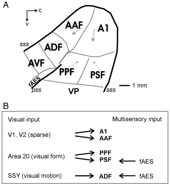
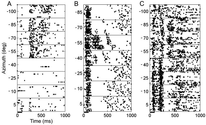
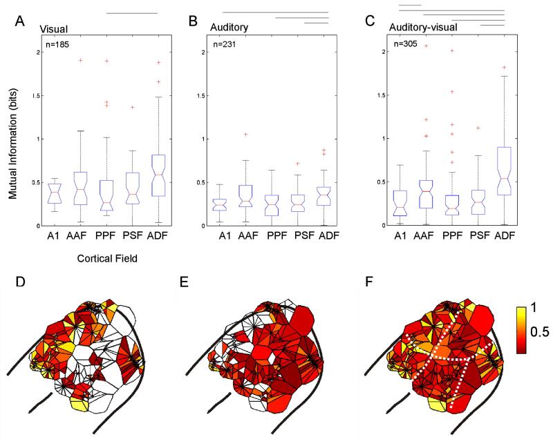
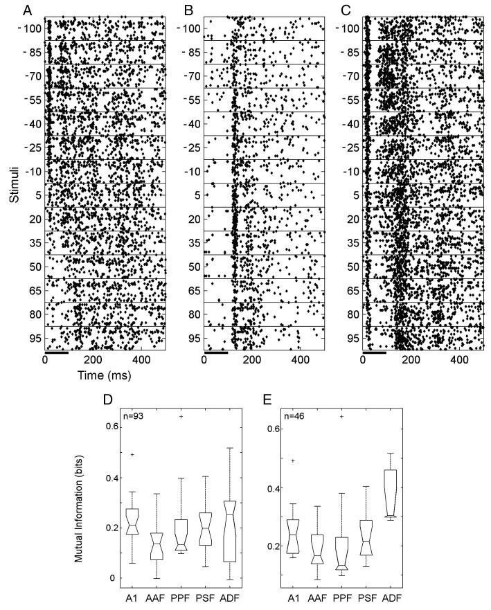
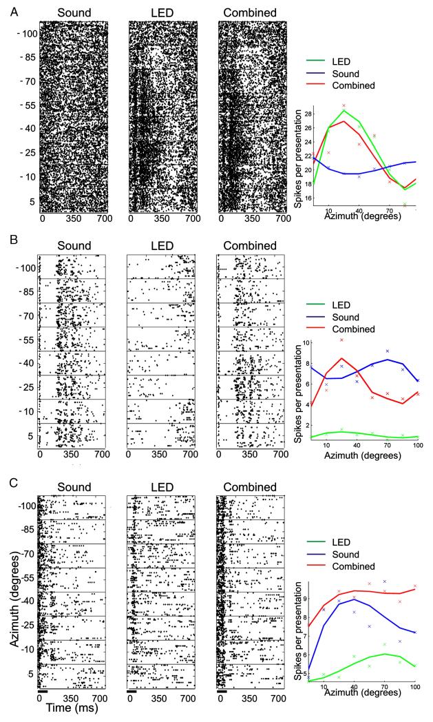
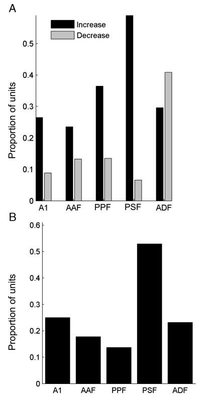
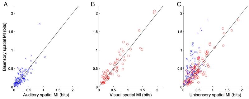
Neurons responsive to visual stimulation have now been described in the auditory cortex of various species, but their functions are largely unknown. Here we investigate the auditory and visual spatial sensitivity of neurons recorded in 5 different primary and non-primary auditory cortical areas of the ferret. We quantified the spatial tuning of neurons by measuring the responses to stimuli presented across a range of azimuthal positions and calculating the mutual information (MI) between the neural responses and the location of the stimuli that elicited them. MI estimates of spatial tuning were calculated for unisensory visual, unisensory auditory and for spatially and temporally coincident auditory-visual stimulation. The majority of visually responsive units conveyed significant information about light-source location, whereas, over a corresponding region of space, acoustically responsive units generally transmitted less information about sound-source location. Spatial sensitivity for visual, auditory and bisensory stimulation was highest in the anterior dorsal field, the auditory area previously shown to be innervated by a region of extrastriate visual cortex thought to be concerned primarily with spatial processing, whereas the posterior pseudosylvian field and posterior suprasylvian field, whose principal visual input arises from cortical areas that appear to be part of the 'what' processing stream, conveyed less information about stimulus location. In some neurons, pairing visual and auditory stimuli led to an increase in the spatial information available relative to the most effective unisensory stimulus, whereas, in a smaller subpopulation, combined stimulation decreased the spatial MI. These data suggest that visual inputs to auditory cortex can enhance spatial processing in the presence of multisensory cues and could therefore potentially underlie visual influences on auditory localization.

Fig. 1

(A) Schematic showing the organization of auditory cortex in the ferret. The primary fields, A1 and AAF, are tonotopically organized (arrows indicate a high-to-low characteristic frequency gradient). Two posterior fields, PPF and PSF, are also tonotopically organized. A1, primary auditory cortex; AAF, anterior auditory field; PPF, posterior pseudosylvian field; PSF, posterior suprasylvian sulcus; VP, ventral posterior; ADF, anterior dorsal field; AVF, anterior ventral field; fAES, anterior ectosylvian sulcal field; pss, pseudosylvian sulcus; sss, suprasylvian sulcus; c, caudal; v, ventral. (B) Summary of visual inputs from visual and multisensory areas into each of the 5 auditory fields recorded from in this study.

Fig. 2

(A–C) Raster plots showing the responses of three units recorded in fields PPF, AAF and ADF, respectively, to light flashes from an LED (100 ms duration) presented at a range of azimuthal locations (at a fixed elevation of + 5°). All three units transmitted significant information about LED location in their response (A, 1.54 bits; B, 2.07 bits; C, 1.59 bits).

Fig. 3

(A–C) Boxplots displaying the amount of information (in bits) transmitted by units in each of the five cortical fields about LED location (A), sound-source location (B) or the location of a combined auditory–visual stimulus (C). Only units for which there was a significant unisensory visual or auditory response are plotted in A and B, respectively, whereas C shows the multisensory MI values for all units recorded, irrespective of their response to unisensory stimulation. The total number of units in each group is shown at the top of each plot. The boxplots show the median (horizontal bar), inter-quartile range (boxes), spread of data (tails) and outliers (cross symbols). The notch indicates the distribution of data about the median. There were significant differences in the distribution of MI values in different cortical fields (Kruskal–Wallis test; LED location, p = 0.0001; auditory location, p = 0.0035; bisensory stimulus location, p < 0.0001). Significant post-hoc pair-wise differences (Tukey–Kramer test, p < 0.05) between individual cortical fields are shown by the lines above each boxplot. (D–F) Voronoi tessellations plotting the spatial information, in bits, on the surface of auditory cortex for every unit recorded. Data from 5 animals have been collapsed onto a single auditory cortex. Each polygon represents a single unit. Where multiple recordings were made at different active sites on the same electrode, recordings are arranged in a circle about the point from which they were recorded. The deepest unit is shown on the right hand side and progressively more superficial units are arranged moving clockwise from this point. Units that conveyed very small amounts of spatial information are plotted in red and the most informative neurons are plotted in yellow.

Fig. 4

(A–C) Raster plots showing the responses of three units to broadband noise bursts (100 ms duration) presented in virtual acoustic space at a range of azimuthal locations (at a fixed elevation of + 5°). All three units transmitted significant information about sound-source location in their responses (0.42, 0.20, and 0.45 bits, respectively). Units A and B were recorded in A1, and unit C in ADF. (D and E) Distribution of MI values obtained from all units tested with this wider range of azimuths (D, n = 93) and from only those units whose responses were significantly spatially modulated (E, n = 48).

Fig. 5

Examples of responses to auditory, visual and combined auditory–visual stimulation. For each unit, the response to the three stimulus types presented at different azimuths is shown by the raster plots and by the spike rate functions (plotted over a 300 ms window and fitted with a cubic polynomial). (A) Unisensory visual unit that was spatially tuned and unaffected by simultaneously presented sound. Spatial MI values obtained for this unit were 0.45, 1.9 and 2.01 bits for acoustic, visual and bisensory stimulation, respectively. (B) Acoustically responsive unit that responded in a consistent fashion across the range of azimuths tested. Unisensory visual stimulation suppressed the spontaneous activity of this unit and, when combined with acoustic stimulation, resulted in a spatially tuned response. Spatial MI values obtained for this unit were 0.31, 0.29 and 0.38 bits for acoustic, visual and bisensory stimulation, respectively. (C) Bisensory unit showing broad spatial tuning to both auditory and visual unisensory stimulation. Pairing auditory and visual stimulation produced a more robust spiking response in this unit, which was modulated much less by spatial location. Spatial MI values obtained for this unit were 0. 49, 0.51 and 0.45 bits for acoustic, visual and bisensory stimulation, respectively.

Fig. 6

(A) Bar graph showing the proportion of units in each cortical field where a significant crossmodal interaction was observed. The proportion of units in which combined auditory–visual stimulation resulted in a significant increase or decrease in spatial information, relative to the most spatially informative unisensory response, is shown by the black and gray bars, respectively. (B) Bar graph plotting the proportion of units within each cortical field in which the addition of a spatially and temporally congruent visual stimulus led to an increase in spatial information compared to that estimated from the response to sound alone.

Fig. 7

Scatter plots plotting the amount of spatial information available from unisensory stimulation (blue crosses, auditory; red circles, visual) against that obtained with bisensory stimulation for units classified as unisensory auditory (A), unisensory visual (B) or bisensory (C).

References

1. Benedek G, Fischer-Szatmari L, Kovacs G, Perenyi J, Katoh YY. Visual, somatosensory and auditory modality properties along the feline suprageniculate-anterior ectosylvian sulcus/insular pathway. Prog. Brain. Res. 1996;112:325–334. - PubMed
1. Bizley JK, Nodal FR, Nelken I, King AJ. Functional organization of ferret auditory cortex. Cereb. Cortex. 2005;15:1637–1653. - PubMed
1. Bizley JK, Nodal FR, Bajo VM, Nelken I, King AJ. Physiological and anatomical evidence for multisensory interactions in auditory cortex. Cereb. Cortex. 2007;17:2172–2189. - PMC - PubMed
1. Brosch M, Selezneva E, Scheich H. Nonauditory events of a behavioral procedure activate auditory cortex of highly trained monkeys. J. Neurosci. 2005;25:6797–6806. - PMC - PubMed
1. Budinger E, Heil P, Hess A, Scheich H. Multisensory processing via early cortical stages: connections of the primary auditory cortical field with other sensory systems. Neuroscience. 2006;143:1065–1083. - PubMed
Publication types