Representation of collective electrical behavior of cardiac cell sheets

Abstract

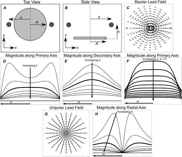
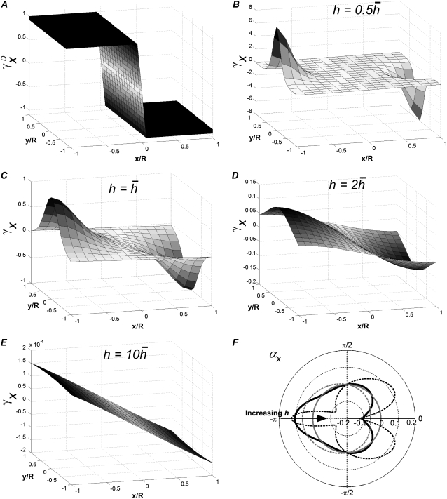
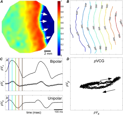
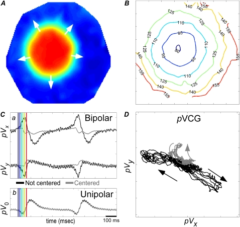
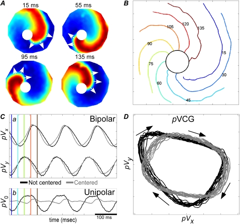
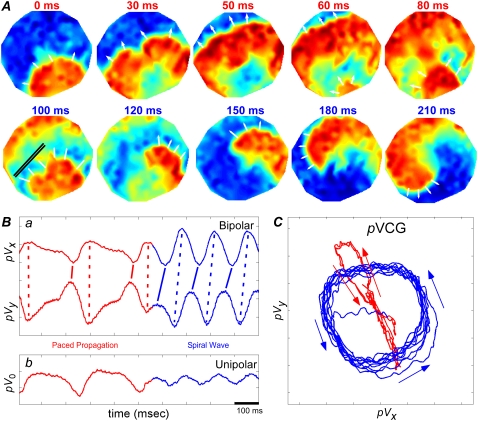
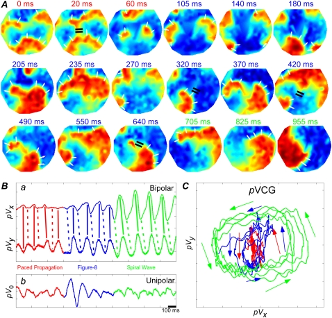
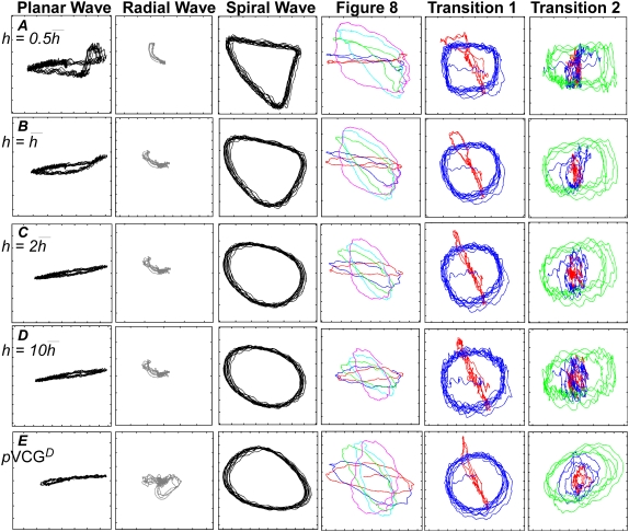
The electrocardiogram (ECG) is a measure of the collective electrical behavior of the heart based on body surface measurements. With computational models or tissue preparations, various methods have been used to compute the pseudo-ECG (pECG) of bipolar and unipolar leads that can be given clinical interpretation. When spatial maps of transmembrane potential (V(m)) are available, pECG can be derived from a weighted sum of the spatial gradients of V(m). The concept of a lead field can be used to define sensitivity curves for different bipolar and unipolar leads and to determine an effective operating height for the bipolar lead position for a two-dimensional sheet of heart cells. The pseudo-vectorcardiogram (pVCG) is computed from orthogonal bipolar lead voltages, which are derived in this study from optical voltage maps of cultured monolayers of cardiac cells. Rate and propagation direction for paced activity, rotation frequency for reentrant activity, direction of the common pathway for figure-eight reentry, and transitions from paced activity to reentry can all be distinguished using the pVCG. In contrast, the unipolar pECG does not clearly distinguish among many of the different types of electrical activity. We also show that pECG can be rapidly computed by two geometrically weighted sums of V(m), one that is summed over the area of the cell sheet and the other over the perimeter of the cell sheet. Our results are compared with those of an ad hoc difference method used in the past that consists of a simple difference of the sum of transmembrane potentials on one side of a tissue sheet and that of the other.

FIGURE 1

(A) Top view of monolayer and (B) side view of monolayer and bipolar lead electrode position. (C) Bipolar lead field, (D) lead field magnitude along primary axis (x axis in A), and (E) secondary axis (y axis in A) of bipolar lead field for increasing h (at a = R). (F) Lead field magnitude along primary axis for increasing a at height (a ≥ R). (G) Unipolar lead field. (H) Lead field magnitude along radial axis of unipolar lead field for increasing h (at a = R). For panels D–H, h is plotted from to in steps of with shown as the bold trace. The case of is also plotted as the dashed trace. For panel F, a is plotted from R to 2R, in steps of 0.1R.

FIGURE 2

Weighting functions for bipolar pECGs. The value γ_x, computed by (A) difference method and (B–E) theoretical method. For panels B–E, and respectively. (F) The value α_x, computed by theoretical method is shown on a polar plot, with radial axis ranging from −0.2 to 0.2. For panel F, (dashed black trace), (solid black trace), (dashed shaded trace), and (shaded trace).

FIGURE 3

(A) Normalized voltage map for planar propagation. The color bar on the right indicates the relative amplitude of V_m (scaled from 0 to 1). (B) Isochrone map. (C) (a) Bipolar pECGs (pV_x and pV_y) and (b) unipolar pECG (pV₀). The colored vertical lines in panel C correspond to isochrones in the isochrone map in panel B. (D) pVCG. Arrows indicate the direction of pVCG with time.

FIGURE 4

(A) Normalized voltage map for radial propagation. (B) Isochrone map. (C) (a) Bipolar pECGs (pV_x and pV_y) for leads placed asymmetrically around (solid traces) or centered on (shaded traces) the stimulus site, and (b) unipolar pECG (pV₀) for lead offset from (solid trace) or centered on (shaded trace) the stimulus site. The shaded trace is covered by the solid trace at nearly all points and is difficult to see. (D) pVCG for bipolar leads placed asymmetrically (solid trace) or symmetrically (shaded trace) around the stimulus site. Different colors for the isochrones in panel B correspond to the instants of time shown in panel C.

FIGURE 5

(A) Normalized voltage maps of spiral wave anchored to 3.5-mm-diameter hole. (B) Isochrone map. (C) (a) Bipolar pECGs (pV_x and pV_y) for leads placed asymmetrically (solid traces) or symmetrically (shaded traces) around hole, and (b) unipolar pECG (pV₀) for lead offset from (solid trace) or centered on (shaded trace) the hole. (D) pVCG for bipolar leads placed asymmetrically (solid trace) or symmetrically (shaded trace) around the hole. Different colors for the isochrones in panel B correspond to the instants of time shown in panel C.

FIGURE 6

(A) Normalized voltage maps of rotating figure-eight reentry. (B) (a) Bipolar pECGs (pV_x and pV_y) and (b) unipolar pECG (pV₀). (C) pVCG. Different colors for the times in panel A correspond to different cycles and are the same as in panels B and C.

FIGURE 7

(A) Normalized voltage maps during transition from paced wave to spiral wave. (B) (a) Bipolar pECGs (pV_x and pV_y) and (b) unipolar pECG (pV₀). Vertical bars have been added to mark the relative timing of the peaks and valleys. (C) pVCG. Different colors in the times in panel A correspond to different propagation patterns and are the same as in panels B and C.

FIGURE 8

(A) Normalized voltage maps during transition from paced wave to figure-eight to spiral wave. (B) (a) Bipolar pECGs (pV_x and pV_y) and (b) unipolar pECG (pV₀). Vertical bars have been added to mark the relative timing of the peaks and valleys. (C) pVCG. Different colors in the times in panel A correspond to different propagation patterns and are the same as in panels B and C.

FIGURE 9

pVCGs calculated at (A) (B) (C) (D) and pVCG^D (E) for six cases of wavefront propagation. The example for the radial wave has been centered. Each plot has been normalized to its own peak amplitude. pVCGs computed at and have unnormalized relative amplitudes of ∼2.5, 1, 0.3, and 0.0042, respectively.

References

-
- Alexander, R. W., J. W. Hurst, and R. C. Schlant. 1994. The Heart, Arteries and Veins. McGraw-Hill, Health Professions Division, New York.
- Burashnikov, A., and C. Antzelevitch. 2003. Reinduction of atrial fibrillation immediately after termination of the arrhythmia is mediated by late phase 3 early afterdepolarization-induced triggered activity. Circulation. 107:2355–2360. - PubMed
- Wu, T. J., S. F. Lin, J. N. Weiss, C. T. Ting, and P. S. Chen. 2002. Two types of ventricular fibrillation in isolated rabbit hearts: importance of excitability and action potential duration restitution. Circulation. 106:1859–1866. - PubMed
- Extramiana, F., and C. Antzelevitch. 2004. Amplified transmural dispersion of repolarization as the basis for arrhythmogenesis in a canine ventricular-wedge model of short-QT syndrome. Circulation. 110:3661–3666. - PubMed
- Skanes, A. C., R. Mandapati, O. Berenfeld, J. M. Davidenko, and J. Jalife. 1998. Spatiotemporal periodicity during atrial fibrillation in the isolated sheep heart. Circulation. 98:1236–1248. - PubMed
Publication types
MeSH terms
Grants and funding
LinkOut - more resources
Full Text Sources
Miscellaneous