The statistical determinants of adaptation rate in human reaching

Abstract

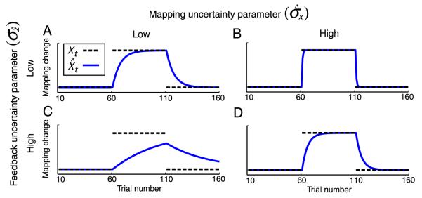
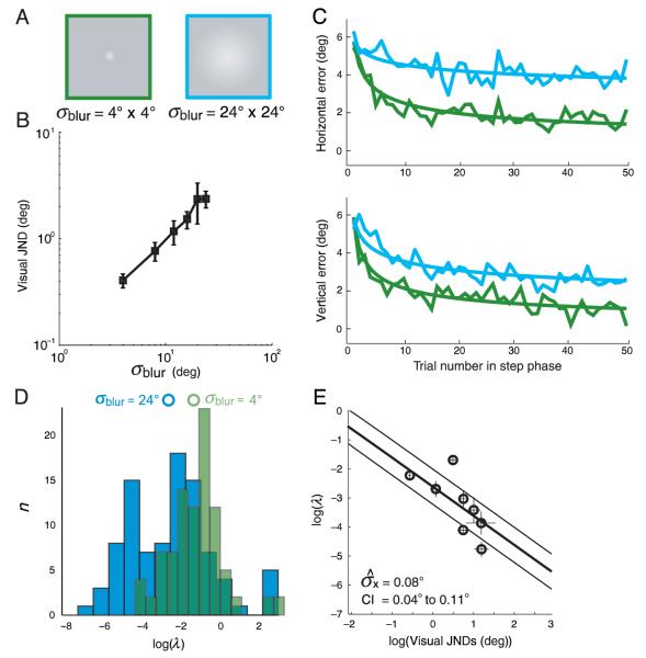
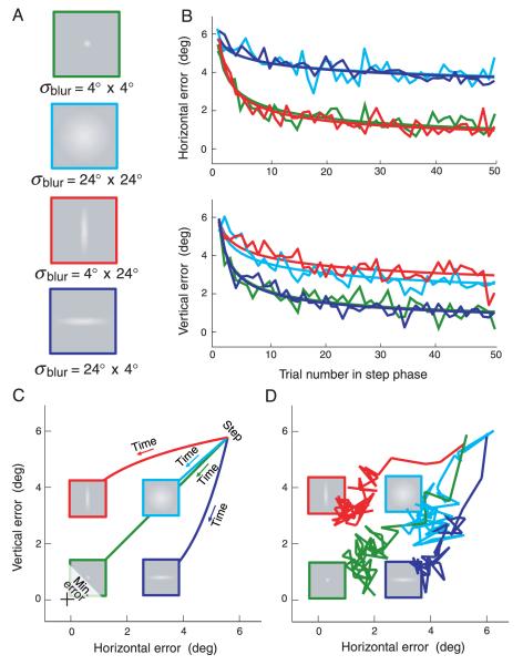
Rapid reaching to a target is generally accurate but also contains random and systematic error. Random errors result from noise in visual measurement, motor planning, and reach execution. Systematic error results from systematic changes in the mapping between the visual estimate of target location and the motor command necessary to reach the target (e.g., new spectacles, muscular fatigue). Humans maintain accurate reaching by recalibrating the visuomotor system, but no widely accepted computational model of the process exists. Given certain boundary conditions, a statistically optimal solution is a Kalman filter. We compared human to Kalman filter behavior to determine how humans take into account the statistical properties of errors and the reliability with which those errors can be measured. For most conditions, human and Kalman filter behavior was similar: Increasing measurement uncertainty caused similar decreases in recalibration rate; directionally asymmetric uncertainty caused different rates in different directions; more variation in systematic error increased recalibration rate. However, behavior differed in one respect: Inserting random error by perturbing feedback position causes slower adaptation in Kalman filters but had no effect in humans. This difference may be due to how biological systems remain responsive to changes in environmental statistics. We discuss the implications of this work.

Figure C1

Efficiency (MSE_filter/MSE_subject) plotted as a function of σ_perturb for different values of σ_walk. (A) Results from Baddeley et al. (2003). When σ_walk was high, efficiency was relatively high and constant as σ_perturb varied. When σ_walk was small, efficiency increased with increasing σ_perturb. The authors argued the latter effect was caused by motor error, which was present in the human data but not in the Kalman filter. (B) Our simulation results. Solid curves: The Kalman filter’s parameter ${\sigma }_{\widehat{z}}$ was equal to σ_perturb, and the simulated subjects’ ${\sigma }_{\widehat{z}}$ was constant. Dashed lines: for comparison, efficiencies from a simulation in which ${\sigma }_{\widehat{z}}$ for both the filter and the simulated subjects was unaffected. Thin lines indicate conditions that Baddeley et al. did not directly test (σ_walk = 0.375 and 1.125 cm). Note the consequence when the feedback uncertainty parameter in the simulated humans is not affected by perturbation but they are modeled as if it is. For a given perturbation variance, MSE_filter will be lower than it otherwise would be, so efficiency will be lower than it should be. The effect is disproportionately larger at large perturbations and therefore could be responsible for the constant efficiency levels at high σ_walk in Baddeley et al. In both simulations, the simulated subject had additive Gaussian motor noise with a standard deviation of 1 cm. In cases in which ${\sigma }_{\widehat{z}}$ was unaffected by σ_perturb, ${\sigma }_{\widehat{z}}$ was set to 0.133 cm, a reasonable value for the visual JND for localizing feedback of the size used in Baddeley et al.

Figure 1

Kalman filter responses to step changes. The dashed black lines in each panel represent the mapping between the position of the reach endpoint and the position of the visual feedback. This relationship is the visuomotor mapping. As in our experiments, there are three phases: pre-step (trials 1–60), step (61–110), and post-step (111–160). A step change in the mapping occurs during the step phase; the initial mapping is restored after the step phase. The blue curves represent the visuomotor mapping estimates (${\widehat{X}}_t$) over time. The upper and lower rows show estimates when the measurement uncertainty (${\sigma }_{\widehat{z}}$) is small and large, respectively. An increase in ${\sigma }_{\widehat{z}}$ causes a decrease in adaptation rate. The left and right columns show responses when the mapping uncertainty (σ_x) is small and large, respectively. An increase in σ_x causes an increase in adaptation rate; the effect is larger when ${\sigma }_{\widehat{z}}$ is large.

Figure 2

Experimental setup and procedure. (A) Experimental setup. Subjects sat in front of a visual display that they viewed binocularly from a distance of 50 cm. Their heads were restrained by a chin-and-forehead rest. Subjects held a stylus with their preferred hand on a horizontal graphics tablet. The hand was not visible. The x—y positions of the stylus were recorded on the tablet. (B) The visual target, actual reach endpoint, and feedback stimulus. Visual feedback was available only at the end of each reach. Reach endpoint was defined as first place the stylus touched the graphics tablet after the reach was initiated. The upper panel shows the target (bright circle), reach endpoint (dashed circle), and visual feedback (bright Gaussian blob superimposed on dashed circle) for trials in which the feedback and endpoint had the pre-step mapping X_t. The lower panel shows the mapping X_t+1 after the mapping change of the step phase: the feedback was displaced by 8.2° up and to the right (5.8° horizontally and 5.8° vertically) relative to the pre-step mapping, as indicated by the offset between the dashed circle and Gaussian blob. A reach error E_t was defined as the difference between the target and the feedback locations. (C) Time course for a trial. The target was presented at a random position for 500 ms. Then, the subject made a rapid reach in response to the target’s position. The position of the reach endpoint was recorded. Then a 500-ms feedback stimulus appeared whose position was determined by the current mapping X_t. (D) Average errors (n = 24) across all three phases (pre-step, step, and post-step) for a single condition. Post-step error reduction was generally faster than step-phase error reduction, but the same basic trends were followed. Because it is advantageous to work with slower rates, we focus our analysis on the step rather than on the post-step data (see Methods for details).

Figure 3

Stimuli and results from Experiment 1. (A) Isotropic visual feedback stimuli. They were isotropic Gaussian blobs with σ_blur = 4° × 4° and 24° × 24°. (B) Just-noticeable differences (JNDs) in the visual localization experiment as a function of σ_blur. Visual discrimination thresholds increased monotonically from 0.4° to 2.4° as σ_blur was increased from 4° to 24°. y = 0.16*x - 0.085, R² = 0.9821. (C) Average adaptation profiles for isotropic feedback stimulus. On the first trial, subjects had no information about the size and the direction of the step, so initial errors were roughly equal to the step. Subjects gradually adjusted their visuomotor mapping estimate, ${\widehat{X}}_t$, so that the observed errors approached zero. Light blue represents the data when σ_blur = 24° × 24° and green represents the data when σ_blur = 4° × 4°. The upper panel plots horizontal error (in degrees) against trial number and the lower panel vertical error (also in degrees) against trial number across trials. One degree corresponds to ∼2.5 mm on the tablet, so the shift of 8.2 deg corresponds to ∼2 cm on the tablet. The line segments represent the data, and the smooth curves are the averages of the best-fitting exponentials (Equation 6). Exponentials and power laws, each with two free parameters, were fit to all individual subject data (exponential: E_t =(b + C)e^-λ(t-1) + b; power: E_t = (b + C)t^-λ + b). Exponentials provided a better fit 78% of the time (p < 1.7*10^-27; sign test, n = 384 (24 subjects × 8 conditions [4° × 4°, 8° × 8°, 12° × 12°, 16° × 16°, 20° × 20°, 24° × 24°, 24° × 4°, and 4° × 24°] × 2 dimensions [x, y])). (D) Histogram of all vertical and horizontal adaptation rates for subjects in which σ_blur was 4° (green) or 24° (light blue) in the respective direction. The histogram includes data from conditions with 4° × 4°, 4° × 24°, 24° × 4°, and 24° × 24° feedback. Rates were significantly slower in the large blur condition (t test, p < .0001; n = 96). (E) Average time constants as a function of average visual JND for each condition of the experiment. Exponential fits were performed along the diagonal (C = 8.2°). This includes the two conditions with anisotropic blobs plotted in Figure 4 and four additional conditions with isotropic blobs (8° × 8°, 12° × 12°, 16° × 16°, and 20° × 20°). Stimuli and data from these conditions are shown in Supplementary Figure 1. Error bars indicate one standard deviation. The thick black line (actually a curve) shows the predicted change of adaptation rate with feedback uncertainty for ${\widehat{\sigma }}_x=0.08°$. The thin black lines are the 95% confidence intervals (R² = 0.61). As ${\widehat{\sigma }}_x$ changes, the y-intercept of the Kalman filter prediction changes, but the slope is effectively unchanged.

Figure 4

Stimuli and results from Experiment 1 comparing anisotropic and isotropic visual feedback conditions. (A) Gaussian blobs with σ_blur = 4° × 4°, 24° × 24°, 4° × 24°, and 24° × 4° used as visual feedback. (B) Average adaptation profiles for isotropic and anisotropic feedback stimuli. Red and dark blue represent the data when the feedback stimulus was anisotropic: σ_blur = 4° × 24° and 24° × 4°, respectively. As in Figure 3, green and light blue represent the data when the feedback was isotropic: σ_blur = 4° × 4° and 24° × 24°, respectively. The upper panel plots horizontal error across trials, and the lower panel plots vertical error across trials. The line segments represent the data, and the smooth curves are the average of the best-fitting exponentials. A repeated measures ANOVA on the best-fitting exponential rates with blur as a factor revealed that the low blur conditions were significantly faster than the high blur conditions (F(1,23) = 54.4, p < .0001). Multiple comparison tests showed that the conditions with low blur in each direction were significantly faster than the high-blur conditions, and that the low-blur conditions did not differ significantly from each other. (C) Spatial profiles for a Kalman filter in response to a step change in the maping. Horizontal error is plotted as a function of vertical error. Initially, the reaching error corresponds to the step change (5.8° horizontally and vertically), so the error is large (upper right). As the filter adjusts its responses over time toward the goal of zero error (lower right), the horizontal and the vertical errors change. When the blur is isotropic (green and light blue), the horizontal and the vertical adaptation rates are the same, so errors progress along a diagonal toward zero error. When the blur is anisotropic (red and dark blue), horizontal and vertical adaptation rates differ, so errors progress along curves, the direction of the curve depending on the direction of least blur. The Kalman filter’s parameter for measurement uncertainty ${\sigma }_{\widehat{z}}$ was set equal to the human visual JNDs for the corresponding conditions. The filter’s parameter for mapping uncertainty ${\widehat{\sigma }}_x$ was set equal to 0.08°, the estimated value of baseline visuomotor mapping uncertainty (see Figure 3E). (D) Spatial profiles for the average human data plotted in the same format.

Figure 5

Stimuli and results from Experiment 2. (A) Example random walks (plus step change) with σ_walk = 0.9° and σ_walk = 2.5°. (B) Reach endpoints multiplied by -1 from two representative subjects (blue traces) in response to two random walks with σ_walk = 0.9° applied to the mapping between reach endpoint and visual feedback positions (solid black traces). Subject mapping estimates clearly followed the walks. The random walks that were added to the step changes were mirror images of one another. The average of the walks was identical to the trial-by-trial stimulus values in Experiment 1 (dashed black trace). Variation due to the walks was nulled by averaging across all walks in Experiment 2. (C) Average adaptation profiles for the random walks during the step phase. Errors are plotted against trial number. Because walk statistics were isotropic within a condition, error was calculated in the direction of the constant shift (rather than in x and y separately). Dark blue: σ_walk = 0.9° × 0.9°; σ_blur = 24° × 24°. Gray: σ_walk = 2.5° × 2.5°, σ_blur = 24° × 24°. Black: σ_walk = 0.9° × 0.9°, σ_blur = 4° × 4°. Orange: σ_walk = 2.5° × 2.5°, σ_blur = 4° × 4°. Walk standard deviation was chosen to be equivalent to the visual JNDs for σ_blur = 4° × 4° and 24° × 24°. The curves are the best-fitting power laws to the data averaged across subjects. Exponentials could not be fit to the individual data because of the drifts associated with the random walks. The rates displayed on the right are the exponents of the best-fitting power laws. An increase in walk variability yields an increase in adaptation rate with large blur. (D) d’ for discriminating adaptation rates as a function of visual JND. Circles indicate the two blur conditions in our experiment. Assuming that the system estimate of mapping uncertainty, ${\widehat{\sigma }}_x$, is roughly equal to σ_walk, rate predictions were made for the two levels of σ_walk imposed in Experiment 2 at multiple blur levels (Equations 4 and 5; Appendix A). Circles mark the blurs tested in Experiment 2. 1000 exponential adaptation profiles were generated with the predicted λ. After corrupting each profile with motor noise (estimated from the pre-step phase of Experiment 1 (σ_motor = ∼2°), we fit each individually with an exponential. d’ was calculated from the resultant distributions of best-fit λs. d’ was 0.2 and 2.6 in the low- and high-blur conditions, respectively. Thus, high rates are difficult to measure reliably because subjects adapt quickly over the first few trials. We therefore do not expect a measurable effect of σ_walk when blur is low.

Figure 6

Results from Experiment 3.(A)Results from Experiment 3a. The insets in panel b represent σ_perturb for the various conditions; σ_blur was fixed at 4° × 4° for all conditions. Black: σ_perturb = 0.9° × 0.9°. Light blue: σ_perturb = 2.5° × 2.5°. Dark blue and red: σ_perturb = 2.5° × 0.9° and 0.9° × 2.5°, respectively. Note that these standard deviations are equivalent to the visual JNDs for the corresponding conditions in Experiment 1. The upper data plot shows horizontal error over trials and the lower plot shows vertical error over trials. The line segments represent the data, and the smooth curves are the averages of the best-fitting exponentials. A repeated measures ANOVA with perturbation as a factor showed no effect of σ_perturb on adaptation rate (F(1,23) = 0.25, p < 0.62). (B) Average spatial profiles of reach errors over trials. Vertical error is plotted as a function of horizontal error as in Figure 4D. The profiles were linear for all forms of random perturbation. Note the different pattern of results in Experiment 1. (C) Stimuli and results from Experiment 3b. The insets represent σ_perturb for the various conditions; σ_blur was varied. Light blue: σ_perturb = 0.9° × 0.9°; σ_blur = 24° × 24°. Dark blue: σ_perturb = 2.5° × 2.5°; σ_blur = 24° × 24°. Black: σ_perturb = 0.9° × 0.9°; σ_blur = 4° × 4°. Red: σ_perturb 2.5° × 2.5°; σ_blur = 4° × 4°. An ANOVA showed there was again no effect of σ_perturb (F(1,23) = 0.19, p < 0.67). Blur continued to produce a main effect (F(1,23) = 14.52, p < 0.0009).

References

1. Adams WJ, Banks MS, van Ee R. Adaptation to three-dimensional distortions in human vision. Nature Neuroscience. 2001;4:1063–1064. [PubMed] [Article] - PubMed
1. Alais D, Burr D. The ventriloquist effect results from near-optimal bimodal integration. Current Biology. 2004;14:257–262. [PubMed] [Article] - PubMed
1. Baddeley RJ, Ingram HA, Miall RC. System identification applied to a visuomotor task: Near-optimal human performance in a noisy changing task. Journal of Neuroscience. 2003;23:3066–3075. [PubMed] [Article] - PMC - PubMed
1. Bedford FL. Constraints on learning new mappings between perceptual dimensions. Journal of Experimental Psychology. 1989;15:232–248.
1. Bedford FL. Perceptual learning. In: Medin D, editor. The psychology of learning and motivation. Academic Press; New York: 1993a. pp. 1–60.
Publication types