The stochastic edge in adaptive evolution

Abstract

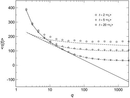
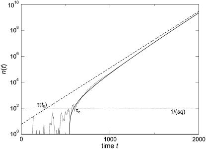
In a recent article, Desai and Fisher proposed that the speed of adaptation in an asexual population is determined by the dynamics of the stochastic edge of the population, that is, by the emergence and subsequent establishment of rare mutants that exceed the fitness of all sequences currently present in the population. Desai and Fisher perform an elaborate stochastic calculation of the mean time tau until a new class of mutants has been established and interpret 1/tau as the speed of adaptation. As they note, however, their calculations are valid only for moderate speeds. This limitation arises from their method to determine tau: Desai and Fisher back extrapolate the value of tau from the best-fit class's exponential growth at infinite time. This approach is not valid when the population adapts rapidly, because in this case the best-fit class grows nonexponentially during the relevant time interval. Here, we substantially extend Desai and Fisher's analysis of the stochastic edge. We show that we can apply Desai and Fisher's method to high speeds by either exponentially back extrapolating from finite time or using a nonexponential back extrapolation. Our results are compatible with predictions made using a different analytical approach (Rouzine et al.) and agree well with numerical simulations.

Figure 1.—

Numerical evaluation of the average in simulations of the stochastic edge, as a function of q, for U_b = 10⁻⁴ and sq = 0.02 held constant throughout. Points are simulation results; the standard error from the simulations is smaller than the symbol size. As measurement times t, we used three multiples of and determined from the approximation formula Equation 57. The dashed lines were calculated from Equation 32 (valid only for large q). The solid line represents (Equation 19, valid for all q).

Figure 2.—

Stochastic-edge simulation and back extrapolation to obtain τ(t₀) and τ_c. The thin solid line represents the size n(t) of the best-fit class in a typical stochastic-edge simulation run for s = 0.001, U_b = 0.0001, and q = 10. The thick solid line is Equation 42 with τ_c = 590 and the dashed line is Equation 4 with τ(t₀) = 284. The values of τ_c and τ(t₀) have been determined at time t₀ = 10,000, which means that the stochastic value n(t₀) is indeed given by, respectively, Equations 42 and 4. For large times (), both fits are good but for intermediate times, the stochastic n(t) is best captured by the thick solid line. The time at which n(t) reaches the stochastic threshold 1/(sq) (represented as a horizontal dotted line) is much closer to τ_c than to τ(t₀). Moreover, the value of τ(t₀) would have depended much more on the choice of t₀. For instance, taking t₀ = 1000 would have given τ(t₀) = 380 and τ_c = 578.

Figure 3.—

Measured values collapse onto a single scaling function F(q). Data points are simulation results obtained from stochastic-edge simulations. For each parameter setting, we measured and then plotted as a function of q. The solid line represents a numerical evaluation of Equation 52 and the dashed line represents the approximate analytic expression Equation 53. The dotted line is the scaling function derived from Equation 57.

Figure 4.—

Speed of adaptation as a function of population size N. Points are simulation results: the solid circles come from stochastic simulations of the full model, while the open diamonds come from semideterministic simulations where only the best-fit class is stochastic. Dashed lines were obtained by numerically solving Equations 36 and 39 of Desai and Fisher (2007). Solid lines were obtained by numerically solving Equations 54 and 60 in the present work. Dotted lines are Equation 52 (for A) and Equation 51 (for B) from Rouzine et al. (2008). Parameters are s = 0.01 and U_b = 10⁻⁵ (A) and s = 0.01 and U_b = 0.002 (B). Note that our simulation results are in excellent agreement with simulation results reported by Desai and Fisher (2007).

References

1. Abate, J., and P. P. Valkó, 2004. Multi-precision laplace transform inversion. Int. J. Numer. Methods Eng. 60 979–993.
1. Athreya, K. B., and P. E. Ney, 1972. Branching Processes. Springer, New York.
1. Baake, E., M. Baake and H. Wagner, 1997. Ising quantum chain is equivalent to a model of biological evolution. Phys. Rev. Lett. 78 559–562.
1. Barton, N. H., 1995. Linkage and the limits to natural selection. Genetics 140 821–841. - PMC - PubMed
1. Beerenwinkel, N., T. Antal, D. Dingli, A. Traulsen, K. W. Kinzler et al., 2007. Genetic progression and the waiting time to cancer. PLoS Comput. Biol. 3 e225. - PMC - PubMed
Publication types