A general framework for the distance-decay of similarity in ecological communities
- PMID: 18494792
- PMCID: PMC2613237
- DOI: 10.1111/j.1461-0248.2008.01202.x
A general framework for the distance-decay of similarity in ecological communities
Abstract
Species spatial turnover, or beta-diversity, induces a decay of community similarity with geographic distance known as the distance-decay relationship. Although this relationship is central to biodiversity and biogeography, its theoretical underpinnings remain poorly understood. Here, we develop a general framework to describe how the distance-decay relationship is influenced by population aggregation and the landscape-scale species-abundance distribution. We utilize this general framework and data from three tropical forests to show that rare species have a weak influence on distance-decay curves, and that overall similarity and rates of decay are primarily influenced by species abundances and population aggregation respectively. We illustrate the utility of the framework by deriving an exact analytical expression of the distance-decay relationship when population aggregation is characterized by the Poisson Cluster Process. Our study provides a foundation for understanding the distance-decay relationship, and for predicting and testing patterns of beta-diversity under competing theories in ecology.
Figures
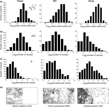
 appear log-normal (in Yasuni) to right-skewed log-normal (in BCI and Korup); plotted on a linear scale, they are characterized by left-skewed shapes similar to those observed by Plotkin et al. (2000) (their fig. 5; see Appendix SE). (b–c) The distributions of number of clumps ρA0 and number of individuals per clump μ vary greatly between forests: species with few clusters and many individuals per cluster are common in Korup, but scarce in Yasuni, where species tend to be clumped in more clusters with fewer individuals. (d) Topographic maps and typical spatial distributions for trees in Yasuni, BCI and Korup.
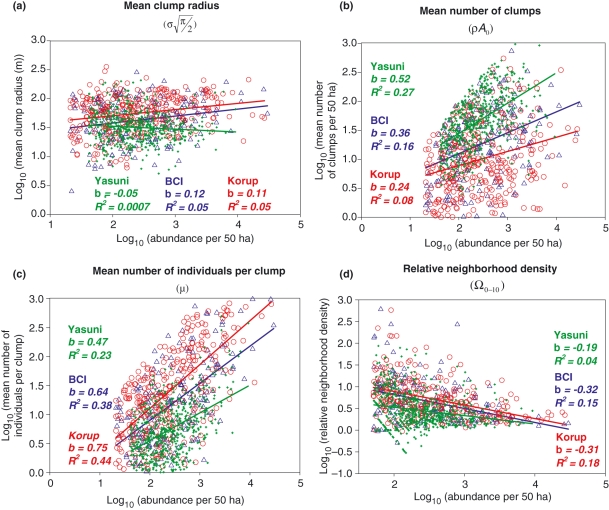
 (b) the number of clumps ρA0, (c) the mean number of individuals per clump μ and (d) the relative neighbourhood density Ω0-10 on a species’ abundance n. All correlations are significant (Spearman test, P < 0.05); b-values correspond to the slope of the log–log regression of the parameters against abundance.
References
-
- Brown JH, Mehlman DW, Stevens GC. Spatial variation in abundance. Ecology. 1995;76:2028–2043.
-
- Chave J, Leigh EG. A spatially explicit neutral model of beta-diversity in tropical forests. Theor. Popul. Biol. 2002;62:153–168. - PubMed
-
- Condit R, Ashton PS, Baker P, Bunyavejchewin S, Gunatilleke S, Gunatilleke N, et al. Spatial patterns in the distribution of tropical tree species. Science. 2000;288:1414–1418. - PubMed
-
- Condit R, Pitman N, Leigh EG, Chave J, Terborgh J, Foster RB, et al. Beta-diversity in tropical forest trees. Science. 2002;295:666–669. - PubMed
Publication types
MeSH terms
LinkOut - more resources
Full Text Sources