. 2009 Apr;30(4):1290-309.
doi: 10.1002/hbm.20597.

Source estimates for MEG/EEG visual evoked responses constrained by multiple, retinotopically-mapped stimulus locations

Affiliations

Source estimates for MEG/EEG visual evoked responses constrained by multiple, retinotopically-mapped stimulus locations

Donald J Hagler Jr et al. Hum Brain Mapp. 2009 Apr.

Abstract

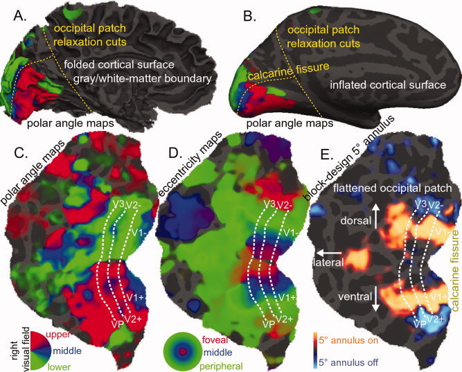
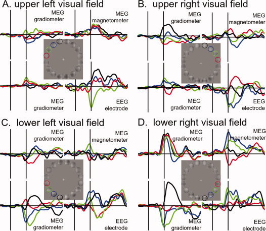
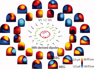
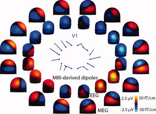
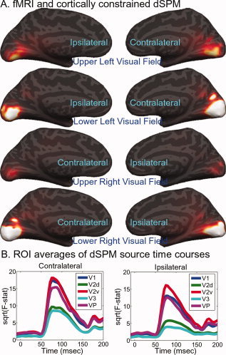
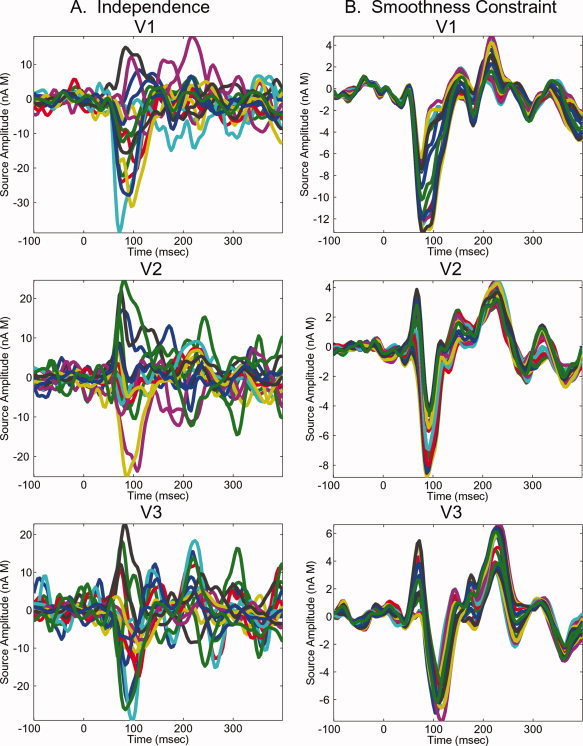
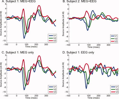
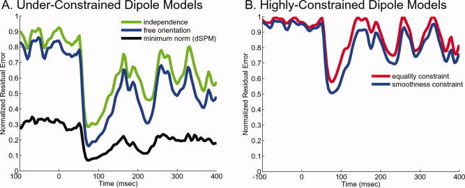
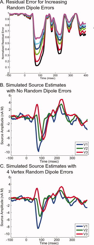
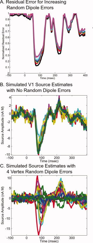
Studying the human visual system with high temporal resolution is a significant challenge due to the limitations of the available, noninvasive measurement tools. MEG and EEG provide the millisecond temporal resolution necessary for answering questions about intracortical communication involved in visual processing, but source estimation is ill-posed and unreliable when multiple; simultaneously active areas are located close together. To address this problem, we have developed a retinotopy-constrained source estimation method to calculate the time courses of activation in multiple visual areas. Source estimation was disambiguated by: (1) fixing MEG/EEG generator locations and orientations based on fMRI retinotopy and surface tessellations constructed from high-resolution MRI images; and (2) solving for many visual field locations simultaneously in MEG/EEG responses, assuming source current amplitudes to be constant or varying smoothly across the visual field. Because of these constraints on the solutions, estimated source waveforms become less sensitive to sensor noise or random errors in the specification of the retinotopic dipole models. We demonstrate the feasibility of this method and discuss future applications such as studying the timing of attentional modulation in individual visual areas.


Figures

Figure 1
Figure 1
Retinotopic maps acquired with 3T fMRI from Subject 1. (A) Polar angle maps superimposed on folded cortical surface (boundary between gray and white‐matter) of left hemisphere. (B) Polar angle maps on inflated cortical surface. (C) Polar angle maps on flattened representation of the left hemisphere occipital cortical surface, with relaxation cuts along the calcarine fissure (shown in A and B as yellow dashed lines). Preferred (contralateral) polar angle is represented by colors indicated by legend. (D) Eccentricity maps. (E) Activation from flashing checkerboard annulus at a fixed eccentricity of 5° (±0.75°) visual angle. 18–22 s “on” blocks alternated with similar blocks of central fixation with no visual stimulation. [Color figure can be viewed in the online issue, which is available at www.interscience.wiley.com.]
Figure 2
Figure 2
MEG/EEG evoked responses to visual stimulation from Subject 1. Signals from two gradiometers, one magnetometer, and an EEG electrode at a mid‐line occipital location. Vertical lines indicate time of stimulus onset and 80‐ms post‐stimulus. Vertical scales are ±60 fT/cm for gradiometers, ± 120 fT for magnetometers, and ±5 μV for EEG electrode (up = positive). Gray squares with colored circles indicate which colored trace corresponds to each stimulus location (n.b., no colored circles were present in the stimuli as presented to the subjects). [Color figure can be viewed in the online issue, which is available at www.interscience.wiley.com.]
Figure 3
Figure 3
MEG and EEG contour plots arranged at polar angles corresponding to 16 iso‐eccentricity stimulus locations. MEG data (average amplitudes over 80‐ to 90‐ms post‐stimulus, gradiometers only) are interpolated onto the helmet surface (outer ring of contour plots) with red representing flux out of the head and blue representing flux into the head. EEG data is interpolated onto the outer scalp surface, with red representing positive scalp potentials and blue representing negative scalp potentials. Dipoles for V1, V2, and V3 (derived from structural and functional MRI data) are represented as ball and stick diagrams with the direction and length of the line indicating the dipole orientation components in the coronal plane. Data are from Subject 1. [Color figure can be viewed in the online issue, which is available at www.interscience.wiley.com.]
Figure 4
Figure 4
Predicted MEG and EEG contour plots for V1. Predicted MEG and EEG data were generated for current dipoles derived from structural and functional MRI (see Methods). Plotting conventions are same as in Figure 3. [Color figure can be viewed in the online issue, which is available at www.interscience.wiley.com.]
Figure 5
Figure 5
Cortically constrained, fMRI‐biased, noise‐normalized, L 2 minimum‐norm source estimates of visual evoked responses. (A) Medial, inflated views of cortical surface overlaid with dSPM statistics (see Methods) for visual responses evoked by stimuli in upper and lower, right and left quarterfields (eccentricity = 5°, polar angles = 56° 124°, 236°, 304°). (B) ROI average time courses for V1, V2, and V3 derived from dSPM. Source estimate statistics were averaged within hand‐drawn cortical surface‐based regions of interest (based on fMRI retinotopy maps and calculated field sign; see Methods), and then collapsed across hemispheres and stimulus locations into averages for contralateral or ipsilateral stimuli. [Color figure can be viewed in the online issue, which is available at www.interscience.wiley.com.]
Figure 6
Figure 6
Retinotopy‐constrained source estimates with independence between stimulus locations or smoothness constraint. Dipole locations were chosen for each stimulus location for V1, V2, and V3, and orientations were fixed to be perpendicular to the cortical surface at each location. (A) Sources waveforms for each stimulus location were estimated independently. (B) Source waveforms were assumed to smoothly vary with stimulus location (see Methods). [Color figure can be viewed in the online issue, which is available at www.interscience.wiley.com.]
Figure 7
Figure 7
Retinotopy‐constrained source estimates assuming equality of source amplitudes across 16 stimulus locations. (A) Source estimates for Subject 1 generated for each visual area, constrained by the MEG and EEG data from the multiple stimulus locations. (B) Source estimates generated from Subject 2's MEG and EEG data (with dipoles modeled from Subject 2's MRI data). (C) Source estimates for Subject 1 using only MEG data. (D) Using only EEG data. [Color figure can be viewed in the online issue, which is available at www.interscience.wiley.com.]
Figure 8
Figure 8
Residual error of visual evoked source estimates. (A) Normalized residual error for underconstrained but regularized (assumed SNR = 1 RMS) source models including (1) retinotopy‐constrained dipole locations and orientations, (2) retinotopy‐constrained dipole locations with free orientations, and (3) L 2 minimum norm (dSPM). All three models allow independence between stimulus locations. (B) Normalized residual error for retinotopy‐constrained source estimates with (1) smoothness constraint, and (2) equality constraint. Normalized residual error was calculated as the ratio between the variance of the residual error and the total variance of the data. [Color figure can be viewed in the online issue, which is available at www.interscience.wiley.com.]
Figure 9
Figure 9
Insensitivity of estimated source waveform to typical errors in modeled dipole orientations with equality constraint. (A) Residual error of simulated source estimates with varying levels of average random dipole orientation errors (0, 18°, 30°, 37°, 41°, and 44°), corresponding to 0–5 vertex distance away from “true” dipole location. (B) Simulated source estimates with no dipole errors. (C) Simulated source estimates with 41° dipole errors, corresponding to ∼4 vertex displacement from “true” location. [Color figure can be viewed in the online issue, which is available at www.interscience.wiley.com.]
Figure 10
Figure 10
Sensitivity of estimated source waveform to typical errors in modeled dipole orientations with independence between stimulus locations. (A) Residual error of simulated source estimates with varying levels of average random dipole orientation errors (0, 18°, 30°, 37°, 41°, and 44°), corresponding to 0–5 vertex distance away from “true” dipole location. (B) Simulated V1 source estimates with no dipole errors. (C) Simulated V1 source estimates with 41° dipole errors, corresponding to ∼4 vertex displacement from “true” location. [Color figure can be viewed in the online issue, which is available at www.interscience.wiley.com.]

Similar articles

Cited by

References

    1. Ahlfors SP,Ilmoniemi RJ,Hamalainen MS ( 1992): Estimates of visually evoked cortical currents. Electroencephalogr Clin Neurophysiol 82: 225–236. - PubMed
    1. Aine CJ,Supek S,George JS,Ranken D,Lewine J,Sanders J,Best E,Tiee W,Flynn ER,Wood CC ( 1996): Retinotopic organization of human visual cortex: Departures from the classical model. Cereb Cortex 6: 354–361. - PubMed
    1. Aine C,Huang M,Stephen J,Christner R ( 2000): Multistart algorithms for MEG empirical data analysis reliably characterize locations and time courses of multiple sources. Neuroimage 12: 159–172. - PubMed
    1. Avidan G,Harel M,Hendler T,Ben‐Bashat D,Zohary E,Malach R ( 2002): Contrast sensitivity in human visual areas and its relationship to object recognition. J Neurophysiol 87: 3102–3116. - PubMed
    1. Barth DS,Di S ( 1991): Laminar excitability cycles in neocortex. J Neurophysiol 65: 891–898. - PubMed

MeSH terms