. 2008 Aug 30;173(2):235-40.
doi: 10.1016/j.jneumeth.2008.06.003. Epub 2008 Jun 17.

Achieving behavioral control with millisecond resolution in a high-level programming environment

Affiliations

Achieving behavioral control with millisecond resolution in a high-level programming environment

Wael F Asaad et al. J Neurosci Methods. .

Abstract

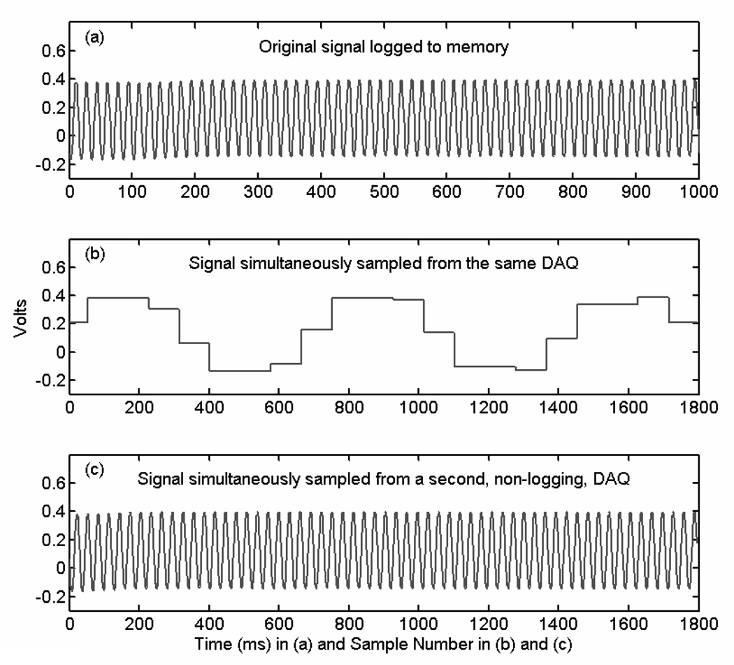
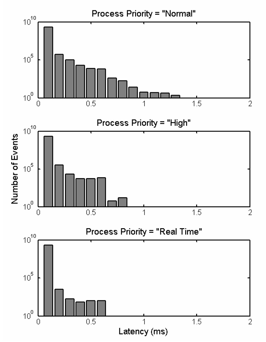
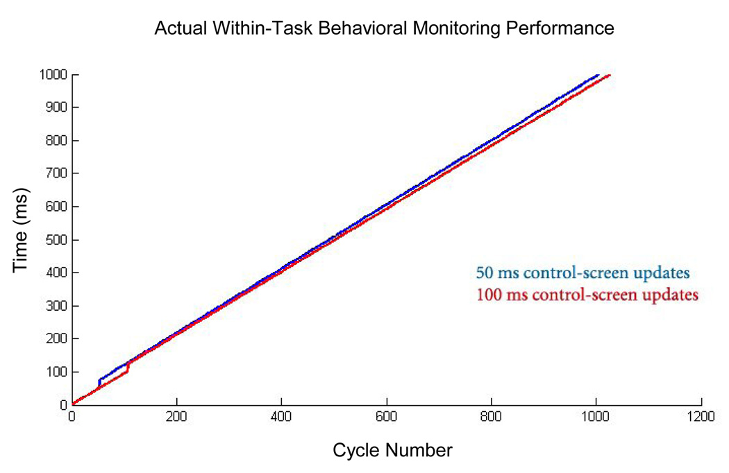
The creation of psychophysical tasks for the behavioral neurosciences has generally relied upon low-level software running on a limited range of hardware. Despite the availability of software that allows the coding of behavioral tasks in high-level programming environments, many researchers are still reluctant to trust the temporal accuracy and resolution of programs running in such environments, especially when they run atop non-real-time operating systems. Thus, the creation of behavioral paradigms has been slowed by the intricacy of the coding required and their dissemination across labs has been hampered by the various types of hardware needed. However, we demonstrate here that, when proper measures are taken to handle the various sources of temporal error, accuracy can be achieved at the 1 ms time-scale that is relevant for the alignment of behavioral and neural events.


Figures

Figure 1
Figure 1. Analog Input Sampling and Aliasing
A 60-Hertz sinusoid resulting from ambient noise was amplified and fed into the data acquisition system. (a) The original signal sampled at 1 kHz as logged to memory. (b) The same signal simultaneously sampled by Matlab as fast as software allowed (~1.8 kHz). (c) The same signal split and fed into a second data acquisition board, sampled while that board was left in a non-logging (“free-running”) state. These figures demonstrate that when an acquisition board is set to log data to memory or disk, that data becomes available to Matlab only after it has been uploaded in chunks to motherboard memory. Attempting to simultaneously sample this data, as in (b), results in the retrieval of the last uploaded data point, even that sample is tens of milliseconds old. This produces an aliased image of the signal which is not adequate for real-time behavioral control. Instead, data sampled from a second acquisition board, set not to log data, provides an accurate, immediate record of the signal. In this way, data can both be logged for post-hoc analysis and used for on-line behavioral control. (d) With the DAQ set to acquire data at 1 kHz, the number of samples uploaded to memory is plotted against time for two settings: the result using the default buffer size set by Matlab is depicted by the dotted line, and result using the minimum allowable buffer size is depicted by the solid line. Shrinking the DAQ’s buffer size provided a significant but limited benefit (gaps between uploads still occurred, lasting about 15 ms). Thus, the two-DAQ solution offered the best performance.
Figure 2
Figure 2. Cycle Rates Achieved on Different Machines
The ranges of observed frequencies at which computers with different levels of processing power were able to execute the behavioral monitoring loop are shown. This loop involves signal sampling, signal calibration, and target-checking. Included here, also, are periodic updates to the control screen (to redraw the position of the eye-trace, visible only to the experimenter), occurring every 50 to 100 ms. A) Intel Pentium 4 running at 2.4 GHz with an 800 MHz FSB. B) Intel Core 2 Duo running at 1.86 GHz with an 800 MHz FSB. C) Intel Core 2 Duo running at 3.4 GHz with an 800 MHz FSB. D) Intel Core 2 Duo running at 3 GHz with a 1333 MHz FSB. Note that the bars around each point represent the approximate observed ranges, not standard deviations. The exact value that would be observed within this range depends on the particular task being run.
Figure 3
Figure 3. Event Timing
The temporal jitter obtained by time-stamping 1000 events, each 100 ms apart. The three dots mark the three occurrences of jitter beyond 0.1 ms, the greatest of which was 1.2 ms late.
Figure 4
Figure 4. Process Priority and OS Delays
Latencies encountered within Matlab at three different process priorities on our test system (see Methods for specifications), each tested over one continuous hour. Latency is plotted against the number of events on a logarithmic scale. Note that as the process priority was increased (the second and third graphs), the distribution of latencies shifted to the left. Concomitant with this decrease in latencies, the number of cycles completed increased from ~566,000 to ~574,000 to ~587,000 as the Matlab priority was increased from “Normal” to “High” to “Real Time.” In no case were there any latencies greater than 1.3 ms. At the highest priority setting, latencies greater than 0.2 ms would be encountered only once every 8.2 seconds, on average. Because of the large number of samples collected over the course of each hour (yielding too many data points to hold all at once in memory), the following procedure was used to generate these graphs: A time-stamp was retrieved at the beginning of each cycle of a loop. The preceding time-stamp was then subtracted from the current one and the difference was rounded to the nearest 0.1 ms. Then, the corresponding bin of a histogram vector encompassing all time differences up to 100 ms (in 0.1 ms steps) was incremented (1000 bins total). Importantly, any delays greater than 100 ms were put into the highest bin so as not to be missed. This vector could then be used to generate directly these bar graphs. These measured latencies, therefore, include these processing steps.
Figure 5
Figure 5. Actual Within-Task Behavioral Monitoring Performance
Plotted here is cycle number versus time, in milliseconds, on our test system (see Methods for specifications). There is a linear relationship between these variables, demonstrating roughly equal time intervals between samples. The one exception to this linearity occurs at the time of the first call for a control-screen update (the issuing of a “drawnow” command at 50 ms for the blue line and 100 ms for the red line); at that time, a gap of approximately 23 milliseconds was measured, meaning the software was blind to changes in the behavioral signal during this time. Importantly, no further such gaps are seen afterward, despite continued calls for updating the control screen at regular 50 or 100 ms intervals. Note that the actual screen update is not expected to occur at these times because of the slower refresh rate (60 Hz) and potential delays within OpenGL (the graphics library used by Matlab). Unlike the subject’s display, the experimenter’s display is low-priority (all that is required is a subjective sense of smooth motion), so these delays were not considered problematic. In contrast to what is depicted here, within our software, this first update is called in the first cycle, thereby fixing the expected “blind” interval to the very beginning of the behavioral tracking period. Note also that there is a slight difference in slope between the 50 and 100 ms conditions, reflecting fewer cycles executed in the former case. This likely reflects added background cost when there is an increased frequency of control screen updates (here, this cost is only on the order of 2 to 3 percent).

References

    1. Ghose GM, Ohzawa I, Freeman RD. A flexible PC-based physiological monitor for animal experiments. J Neurosci Methods. 1995;62:7–13. - PubMed
    1. Hays AV, Richmond BJ, Optican LM. A UNIX-based multiple-process system for real-time data acquisition and control; WESCON Conference Proceedings; 1982. pp. 1–10.
    1. Maunsell JHR. LabLib. 2008. http://maunsell.med.harvard.edu/software.html.
    1. Meyer T, Constantinidis C. A software solution for the control of visual behavioral experimentation. J Neurosci Methods. 2005;142:27–34. - PubMed
    1. Ramamritham K, Shen C, Sen S, Shirgurkar S. Using Windows NT for Real-Time Applications: Experimental Observations and Recommendations; IEEE Real Time Technology and Applications Symposium; 1998.

Publication types

MeSH terms

LinkOut - more resources