Estimating cerebral oxygen metabolism from fMRI with a dynamic multicompartment Windkessel model

Abstract

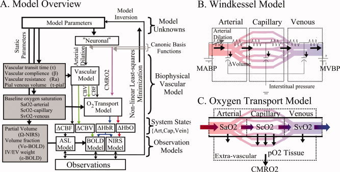
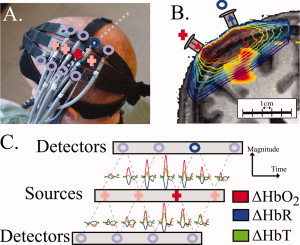
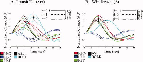
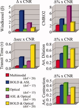
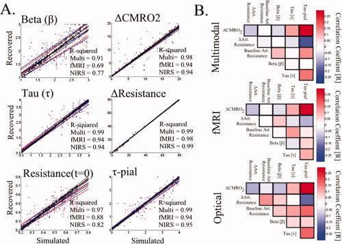
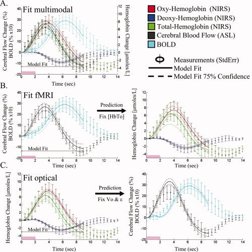
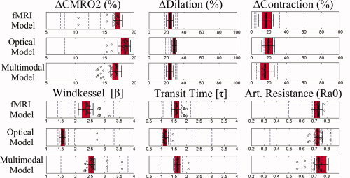
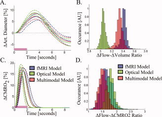
Stimulus evoked changes in cerebral blood flow, volume, and oxygenation arise from responses to underlying neuronally mediated changes in vascular tone and cerebral oxygen metabolism. There is increasing evidence that the magnitude and temporal characteristics of these evoked hemodynamic changes are additionally influenced by the local properties of the vasculature including the levels of baseline cerebral blood flow, volume, and blood oxygenation. In this work, we utilize a physiologically motivated vascular model to describe the temporal characteristics of evoked hemodynamic responses and their expected relationships to the structural and biomechanical properties of the underlying vasculature. We use this model in a temporal curve-fitting analysis of the high-temporal resolution functional MRI data to estimate the underlying cerebral vascular and metabolic responses in the brain. We present evidence for the feasibility of our model-based analysis to estimate transient changes in the cerebral metabolic rate of oxygen (CMRO(2)) in the human motor cortex from combined pulsed arterial spin labeling (ASL) and blood oxygen level dependent (BOLD) MRI. We examine both the numerical characteristics of this model and present experimental evidence to support this model by examining concurrently measured ASL, BOLD, and near-infrared spectroscopy to validate the calculated changes in underlying CMRO(2).

Figure 1

Schematic outline of the vascular model. A vascular forward model (Panel A) based on a multicompartment Windkessel (Panel B) and oxygen transport model (Panel C) is used to estimate the changes in blood flow, volume, and oxygenation in the arterial, capillary, and venous compartments. The model of hemodynamic signals is evoked by underlying changes in vascular tone via arterial vasodilatation and changes in the cerebral metabolic rate of oxygen (CMRO₂). Observation models depicting the biophysics of the optical and fMRI techniques relate the internal states of the model to the measurable hemodynamic responses, which are compared with experimental data.

Figure 2

Optical imaging setup. In this figure, we illustrate the setup used for NIRS recordings. Further details can be found in [Huppert et al., 2006b]. Panel (A) shows the location of the optical probe over the motor cortex for a example subject. The “+” indicate the locations of the light source fibers and “o” indicate the detector fiber positions. In Panel (B) is shown a coronal cross‐section of the subjects anatomical MRI with the fiber positions and measurement sensitivity profiles (contour plot) overlain as described in Huppert et al. [2006a]. The BOLD response (thresh held at P < 0.05) is also overlain on the anatomical image. The dotted line in Panel A shows the approximate location of this slice. In Panel (C) is shown the averaged evoked hemoglobin responses from the performance of the motor task. The locations of the axis indicate the originating pair of source and detector positions for the plotted response.

Figure 3

Parameter sensitivity of the evoked hemodynamic response. This figure illustrates the effect of the biomechanical properties of the vascular network on the temporal dynamics of evoked response. Panels (A) and (B) show qualitatively how the simulated evoked responses vary with different values for the mean vascular transit time (τ) and Windkessel parameter (β). The magnitudes of the responses are normalized to the peak response for each measurement type in order to facilitate cross‐modality comparisons.

Figure 4

Variance inflation factors for model parameters. The lower bound on the uncertainty of each model parameter can be estimated from the variance inflation factor (Γ; described in the text). This factor determines the minimum parameter uncertainty obtainable for a fit of the fMRI, NIRS, or multimodal data. The values in this figure are normalized to the maximum response contrast per modality in order to compare across the various forms of contrast. Thus, the lower bound of the parameter uncertainty for any of the parameters can be estimated for a given contrast‐to‐noise ratio (CNR) by dividing by the CNR value (e.g., with a CNR of 20:1, the Windkessel parameter, β, can be estimated with a maximum precision of around ±0.2 StdErr using the BOLD and ASL data). The degrees‐of‐freedom (dof) for each model is given in the legend. These results are shown for a linearization about the parameter set from the model fit of the multimodal data shown in Table IV.

Figure 5

Examination of global parameter identifiability. In Panel (A), we show the results from 350 simulations of the model. fMRI and NIRS measurements were simulated at a contrast‐to‐noise ratio of 10:1. The vascular parameters (refer to Table III) were estimated from the multimodal (optical and fMRI), fMRI, or optical data sets. For each plot, the simulated and recovered values are shown (black—multimodal; red—fMRI; blue—NIRS). The solid and dotted lines show a linear regression and 95% confidence bounds. The R‐squared (R ²) values for these regressions are shown within each plot. In Panel (B), we examine the cross‐talk between each parameter by looking at the cross‐correlation (Pearson correlation coefficients) of the error in the parameter (normalized error = [recovered‐simulated]/simulated).

Figure 6

Model fit of empirical data. The vascular model was independently fit to the multimodal (Panel A), pulsed ASL and BOLD measurements (Panel B), and NIRS measurements (Panel C). Based on the parameters estimated from the model fit to one data set (i.e., fMRI alone), the remaining data (i.e., NIRS) can be predicted. These model predictions are presented for the fMRI and optical data in Rows B and C. The error bars on the data measurements (open circles) show the standard error from the group average of the five subjects. The model predictions and 75% confidence bounds are shown as solid and dashed lines in each plot. The data from 0 to 9 s was used in the model fitting procedure.

Figure 7

Parameter accuracy. The mean and uncertainties in the parameter estimates are illustrated using box and whisker plots to show the median (vertical line), 50% (box edges), and 75% (whiskers) percentile confidence bounds for each estimated parameter for the model fits to the group averaged data (N = 5). The results are shown for the model fits to the fMRI‐BOLD/ASL data alone, optical NIRS data alone; and multimodal BOLD/ASL/NIRS data sets. The open circles represent the fitted model parameters from variation of the initial starting position of the LM algorithm used in the analysis of the group averaged data (from variations of the extrema of the parameter bounds given in Table III). In addition, the dotted vertical lines show the mean estimates for each of the five individual subjects fit using the same model.

Figure 8

Dynamic CMRO₂ and arterial diameter changes. The dynamic changes in arterial diameter (inversely related to resistance changes) and CMRO₂ are shown in Panels (A) and (C), respectively. The solid and dotted lines show the most probable and 75% confidence intervals for the time‐courses estimated from the multimodal, fMRI, and optical data sets. Panel (B) shows the histogram of the ratio of maximum flow to volume changes recovered from the Markov Chain Monte Carlo process. In Panel (D), the flow‐consumption ratio is shown for the three data sets.

References

1. Bamber D,van Santen JP ( 2000): How to assess a model's testability and identifiability. J Math Psychol 44: 20–40. - PubMed
1. Belliveau JW,Kennedy DN Jr,McKinstry RC,Buchbinder BR,Weisskoff RM,Cohen MS,Vevea JM,Brady TJ,Rosen BR ( 1991): Functional mapping of the human visual cortex by magnetic resonance imaging. Science 254: 716–719. - PubMed
1. Boas DA,Strangman G,Culver JP,Hoge RD,Jasdzewski G,Poldrack RA,Rosen BR,Mandeville JB ( 2003): Can the cerebral metabolic rate of oxygen be estimated with near‐infrared spectroscopy? Phys Med Biol 48: 2405–2418. - PubMed
1. Boxerman JL,Bandettini PA,Kwong KK,Baker JR,Davis TL,Rosen BR,Weisskoff RM ( 1995): The intravascular contribution to fMRI signal change: Monte Carlo modeling and diffusion‐weighted studies in vivo. Magn Reson Med 34: 4–10. - PubMed
1. Buxton RB,Uludag K,Dubowitz DJ,Liu TT ( 2004): Modeling the hemodynamic response to brain activation. Neuroimage 23( Suppl. 1): S220–S233. - PubMed
Publication types