Human vergence eye movements to oblique disparity stimuli: evidence for an anisotropy favoring horizontal disparities

Abstract

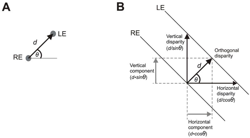
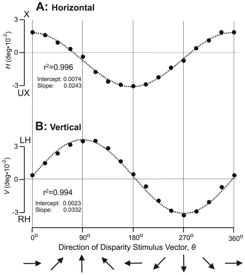
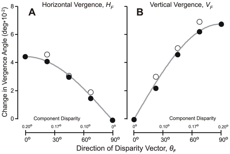
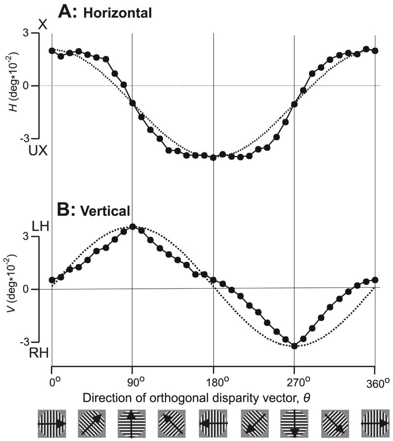
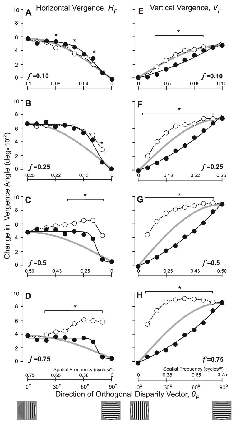
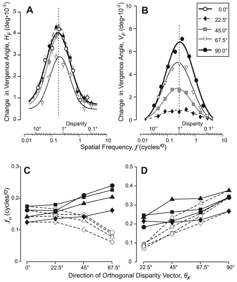
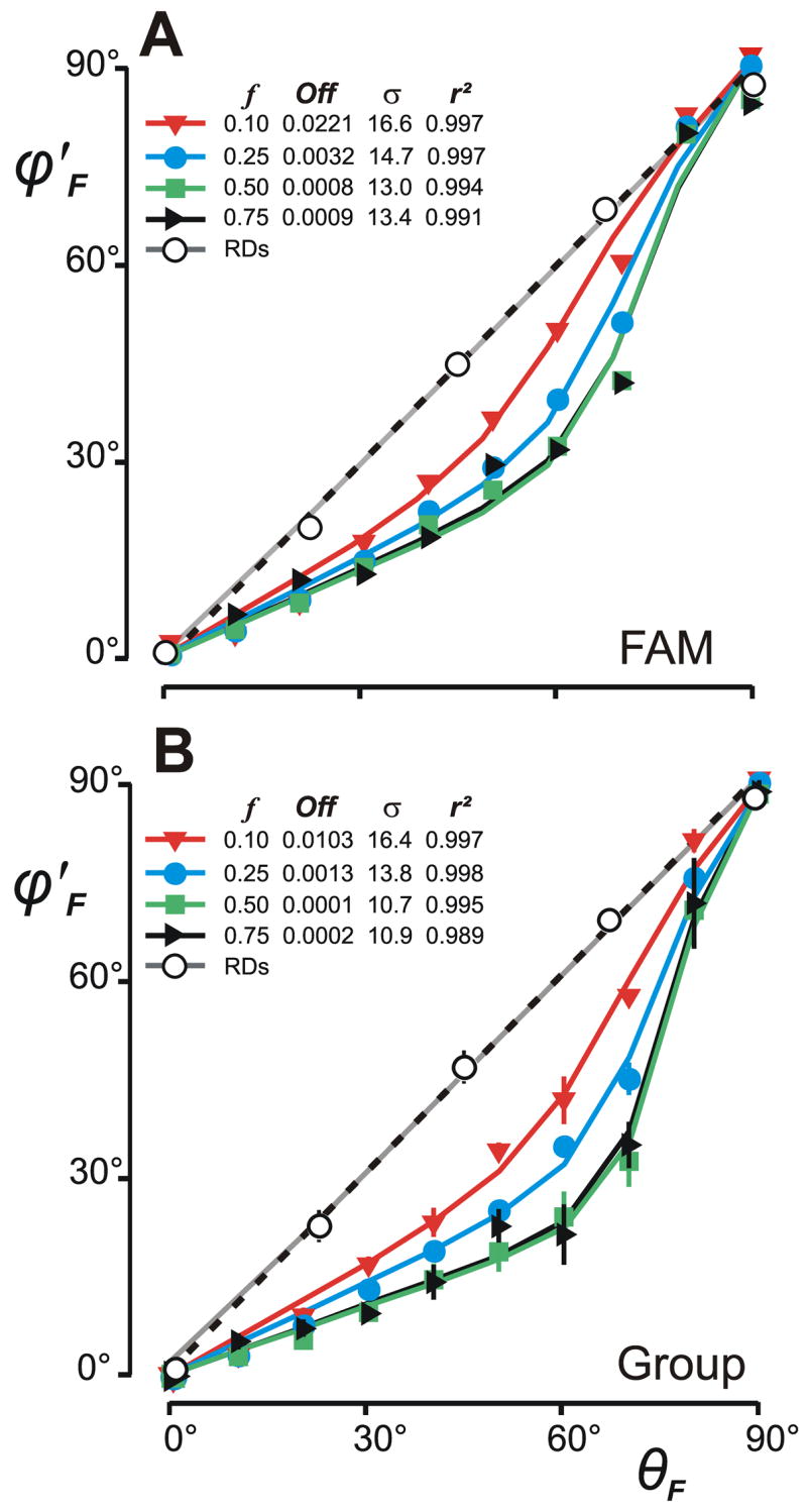
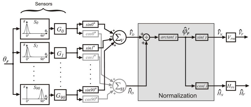
Binocular disparities applied to large-field patterns elicit vergence eye movements at ultra-short latencies. We used the electromagnetic search coil technique to record the horizontal and vertical positions of both eyes while subjects briefly viewed (150 ms) large patterns that were identical at the two eyes except for a difference in position (binocular disparity) that was varied in direction from trial to trial. For accurate alignment with the stimuli, the horizontal and vertical disparity vergence responses (HDVRs, VDVRs) should vary as the sine and cosine, respectively, of the direction of the disparity stimulus vector. In a first experiment, using random-dots patterns (RDs) with a binocular disparity of 0.2 degrees , this was indeed the case. In a second experiment, using 1-D sine-wave gratings with a binocular phase difference (disparity) of 1/4-wavelength, it was not the case: HDVRs were maximal when the grating was vertical and showed little decrement until the grating was oriented more than approximately 65 degrees away from vertical, whereas VDVRs were maximal when the grating was horizontal and began to decrement roughly linearly when the grating was oriented away from the horizontal. We attribute these complex directional dependencies with gratings to the aperture problem, and the HDVR data strongly resemble the stereothresholds for 1-D gratings, which are minimal when the gratings are vertical and remain constant for orientations up to approximately 80 degrees away from the vertical when expressed as spatial phase disparities [Morgan, M. J., & Castet, E. (1997). The aperture problem in stereopsis. Vision Research, 37, 2737-2744.]. To explain this constancy of stereothresholds, Morgan and Castet (1997) postulated detectors sensitive to the phase disparity of the gratings seen by the two eyes (rather than their linear separation along some fixed axis, such as the horizontal). However, because (1) our VDVR data with gratings did not show this constancy and (2) the available evidence strongly suggests that there are no major differences in the disparity detectors mediating the initial HDVR and VDVR, we sought an alternative explanation for our data. We show that the dependence of the initial HDVR and VDVR on grating orientation can be successfully modeled by a bias in the number and/or efficacy of the detectors that favors horizontal disparities.

Figure 1

Disparity stimulus vectors (definitions). (A) Two random dot patterns, identical except for a difference in position of 0.2°, were viewed dichoptically, but here we show only a single pair of corresponding dots; the disparity vector, given by the position of the dot seen by the left eye, LE, with respect to the position of the dot seen by the right eye, RE, had a magnitude of, d, that was fixed (0.2°), and a direction, θ°, measured counterclockwise from the horizontal, that varied from trial to trial. (B) Two 1-D sine-wave grating patterns, identical except for a phase difference of ¼-wavelength, were viewed dichoptically, but here we show only a single pair of corresponding iso-luminance lines; the disparity vector, given by the position of a point on the line seen by the left eye, LE, with respect to its nearest neighbor on the line seen by the right eye, RE, had a magnitude, d, that was fixed (¼-wavelength) and a direction, θ°, orthogonal to the grating and measured counterclockwise from the horizontal, that varied from trial to trial: termed “the orthogonal disparity”; the “horizontal disparity” (d/cosθ) and “vertical disparity” (d/sinθ) refer to the horizontal and vertical separations of the gratings seen by the two eyes; the “horizontal component disparity” (d*cosθ) and “vertical component disparity” (d*sinθ) refer to the horizontal and vertical components of the “orthogonal disparity vector”.

Figure 2

The initial vergence responses when a 0.2° disparity was applied to random dot patterns: dependence of response measures on the direction of the disparity vector, θ (subject FAM). (A) Mean changes in horizontal vergence, H, in filled symbols; convergent responses are positive; X, crossed disparity; UX, uncrossed disparity. (B) Mean changes in vertical vergence, V, in filled symbols; left-sursumvergent responses are positive; LH, left-hyper disparity; RH, right-hyper disparity. Dotted curves are least squares best-fit plots of a+(b*cosθ) in (A) and a+(b*sinθ) in (B), where a and b are free parameters. Each datum point is the mean response to 110–120 repetitions of the stimulus. Standard errors of the means were smaller than the symbols (range: 0.0008–0.0011°).

Figure 3

The initial vergence responses when oblique disparities were applied to random-dot patterns: dependence of the folded response measures on the direction of the folded disparity vector, θ_F (subject FAM). (A) Mean changes in horizontal vergence, H_F; data in filled symbols were obtained with oblique disparity vectors with a magnitude of 0.2°; data in open symbols were obtained with pure horizontal disparity vectors that matched the horizontal components of the oblique disparity vectors, and the magnitudes of their disparities, in degrees, are given on the abscissas above the axis (note: values increase to the left); grey curves are the values of H_F given by H_F0cosθ_F. (B) Mean changes in vertical vergence angle, V_F; data in filled symbols were obtained with oblique disparity vectors with a magnitude of 0.2°; data in open symbols were obtained with pure vertical disparity vectors that matched the vertical components of the oblique disparity vectors, and the magnitudes of their disparities, in degrees, are given on the abscissas above the axis; grey curves are the values of V_F given by V_F90sin θ_F.

Figure 4

The initial vergence responses when 1-D sine-wave gratings (0.25 cycles/°) had a binocular disparity of 1/4–wavelength: dependence of response measures on the direction of the orthogonal disparity vector, θ (subject FAM). (A) Mean changes in horizontal vergence angle, H, in filled symbols; convergent responses are positive; X, crossed disparity; UX, uncrossed disparity. (B) Mean changes in vertical vergence angle, V, in filled symbols; left-sursumvergent responses are positive; LH, left-hyper disparity; RH, right-hyper disparity. Dotted curves are plots of a+(b*cosθ) in (A) and a+(b*sinθ) in (B), where a and b are free parameters and the functions are forced through the data peaks. Cartoons at bottom show sample grating patterns and the arrows indicate the directions of the orthogonal disparity vectors. Each datum point is the mean response to 203–304 repetitions of the stimulus. Standard errors of the means were smaller than the symbols (range: 0.0006–0.0015°).

Figure 5

The initial vergence responses when 1-D sine-wave gratings (0.25 cycles/°) had a binocular disparity of 1/4–wavelength: dependence of the folded response measures on the direction of the (folded) orthogonal disparity vector, θ_F (subject FAM). (A–D) Mean changes in horizontal vergence, H_F; data in filled symbols were obtained with obliquely oriented gratings with orthogonal spatial frequencies (f) of 0.1, 0.25, 0.5, and 0.75 cycles/°; the black lines show the least-squares best fits to these data obtained with Expression 1 (sigmoid function); data in open symbols linked by dashed lines were obtained with vertical gratings whose spatial frequencies matched the horizontal spatial frequencies of the oblique gratings (values, in cycles/°, are given on the abscissas above the axes, and increase in value to the left); grey curves are the values of H_F given by H_F0cos θ_F. (E–H) Mean changes in vertical vergence, V_F; data in filled symbols were obtained with obliquely oriented gratings with orthogonal spatial frequencies (f) of 0.1, 0.25, 0.5, and 0.75 cycles/°; the black lines show the least-squares best fits to these data obtained with Expression 2 (exponential function); data in open symbols linked by dashed lines were obtained with horizontal gratings whose spatial frequencies matched the vertical spatial frequencies of the oblique gratings (values, in cycles/°, are given on the abscissas above the axes); grey curves are the values of V_F given by V_F90sin θ_F. Asterisks indicate those data obtained with oblique gratings (closed symbols) that were significantly different (p<0.05, t-test) from the data obtained with matching cardinal gratings (open symbols). Cartoons at bottom show sample grating patterns. Standard errors of the means were smaller than the symbols (range: 0.0008–0.0034°).

Figure 6

The initial vergence responses when 1-D sine-wave gratings had a binocular disparity of 1/4–wavelength: dependence of the folded response measures on the orthogonal spatial frequency of the grating (in cycles/°) when the orthogonal disparity vector (θ_F) had one of five (folded) directions. (A) Mean changes in horizontal vergence, H_F, as θ_F was fixed at 0°(open circles), 22.5°(diamonds), 45°(squares), and 67.5°(triangles); curves show the least-squares best fit Gaussian functions whose parameters are listed in Table 3; vertical dashed line is aligned on the peak of the Gaussian for which θ_F=0°; subject FAM. (B) Mean changes in vertical vergence, V_F, as θ_F was fixed at 22.5°(diamonds), 45°(squares), 67.5°(triangles), and 90°(closed circles); curves show the least-squares best fit Gaussian functions whose parameters are listed in Table 4; vertical dashed line is aligned on the peak of the Gaussian for which θ_F=90°; subject FAM. (C) Closed symbols show the spatial frequency at the peak of the best-fit Gaussian function (f_o)—based on fits like those in (A)—as a function of the direction of the (folded) orthogonal disparity vector, θ_F, for all four subjects: FAM (squares), BMS (circles), HAR (triangles), and ST (diamonds); open symbols as for the closed symbols except that spatial frequency was specified with respect to the horizontal axis. (D) As in (C) except based on V_F measures like those in (B), and open symbols show data when spatial frequency was specified with respect to the vertical axis.

Figure 7

Directional Decoding “Errors”: dependence of the direction of the normalized folded vergence response vectors, φ′_F, on the direction of the (folded) disparity vector, θ_F. (A) Data for subject, FAM. (B) Mean data (±SD) for four subjects. Closed symbols show data obtained with sine-wave gratings using the orthogonal disparity vector (see key for spatial frequencies). Open circles show data obtained with random-dot patterns. Curves are least-squares best fits obtained with the anisotropy model; the parameters of the Gaussian functions specifying the distributions of the preferred directions of the disparity sensors in the model are listed together with the Coefficients of Determination (r²): f, spatial frequency; Off, vertical offset; σ, standard deviation. Dashed lines are the unity-slope lines.

Figure 8

A block diagram of the anisotropy model. The individual disparity sensors have a Gaussian dependence on the direction of the disparity vector (measured orthogonal to the orientation of the stimulus grating) and all sensors have the same peak response amplitude and bandwidth. The preferred directions of these sensors are arranged in order at 1° intervals (S₀…S₉₀). The gains of the sensor outputs (G₀…G₉₀) have a Gaussian distribution centered on the G₀ element with a width and vertical offset that are free parameters. The outputs of the sensor gain elements, each weighted by the cosine (sine) of its preferred direction, are summed by the horizontal (vertical) vergence premotor controllers, Σ_H (Σ_V), to produce the horizontal (vertical) drive signals, Ĥ_D(V̂_D). A normalization stage then uses simple geometry, given by arctan (V̂_D/Ĥ_D), to derive a signal equivalent to the normalized folded response direction, ${\widehat{\phi }}_F^{\prime }$, which is then decomposed into cosine and sine components, Ĥ_N (V̂_N), that are scaled by the two measured parameters, H_F0 and V_F90, to produce outputs encoding the horizontal and vertical vergence responses: ${\widehat{H}}_F=H_{F0}cos{\widehat{\phi }}_F^{\prime }$ and ${\widehat{V}}_F=H_{F90}sin{\widehat{\phi }}_F^{\prime }$.

References

1. Anzai A, Ohzawa I, Freeman RD. Neural mechanisms for processing binocular information II. Complex cells. Journal of Neurophysiology. 1999;82:909–924. - PubMed
1. Brainard DH. The Psychophysics Toolbox. Spatial Vision. 1997;10:433–436. - PubMed
1. Bridge H, Cumming BG, Parker AJ. Modeling V1 neuronal responses to orientation disparity. Visual Neuroscience. 2001;18:879–891. - PubMed
1. Busettini C, FitzGibbon EJ, Miles FA. Short-latency disparity vergence in humans. Journal of Neurophysiology. 2001;85:1129–1152. - PubMed
1. Busettini C, Miles FA, Krauzlis RJ. Short-latency disparity vergence responses and their dependence on a prior saccadic eye movement. Journal of Neurophysiology. 1996;75:1392–1410. - PubMed
Publication types