

doi: 10.1016/j.jneumeth.2008.07.014.
Epub 2008 Jul 25.
A flexible software tool for temporally-precise behavioral control in Matlab
Affiliations
- PMID: 18706928
- PMCID: PMC2630513
- DOI: 10.1016/j.jneumeth.2008.07.014
Item in Clipboard
A flexible software tool for temporally-precise behavioral control in Matlab
J Neurosci Methods.
.
Abstract
Systems and cognitive neuroscience depend on carefully designed and precisely implemented behavioral tasks to elicit the neural phenomena of interest. To facilitate this process, we have developed a software system that allows for the straightforward coding and temporally-reliable execution of these tasks in Matlab. We find that, in most cases, millisecond accuracy is attainable, and those instances in which it is not are usually related to predictable, programmed events. In this report, we describe the design of our system, benchmark its performance in a real-world setting, and describe some key features.
Figures
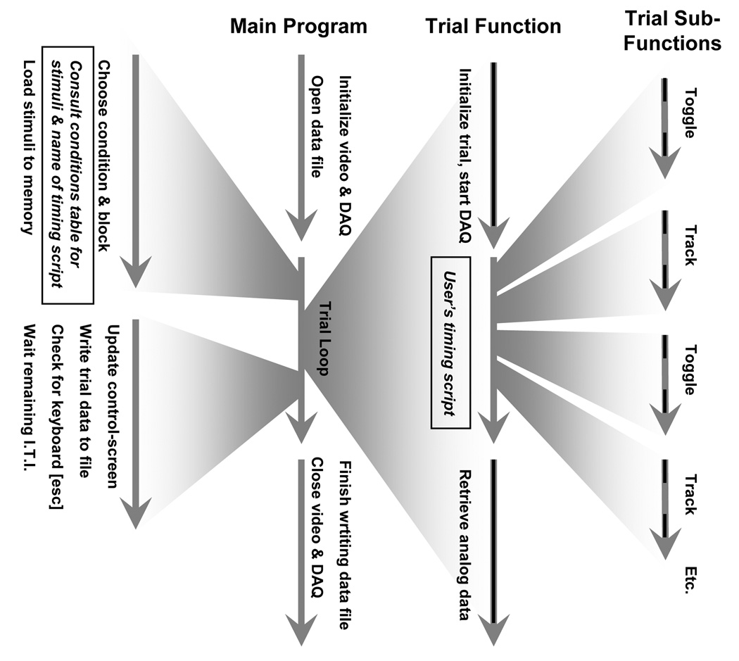
The minimum elements that must be provided by the user are marked with boxes. In addition, user’s can write Matlab scripts to control the time at which blocks change, the selection of blocks, and the selection of conditions. The darker portions of the arrows correspond to the “entry” and “exit” times measured in Table 1 (the eventmarker function is not shown, but would appear intermixed with toggle and track).
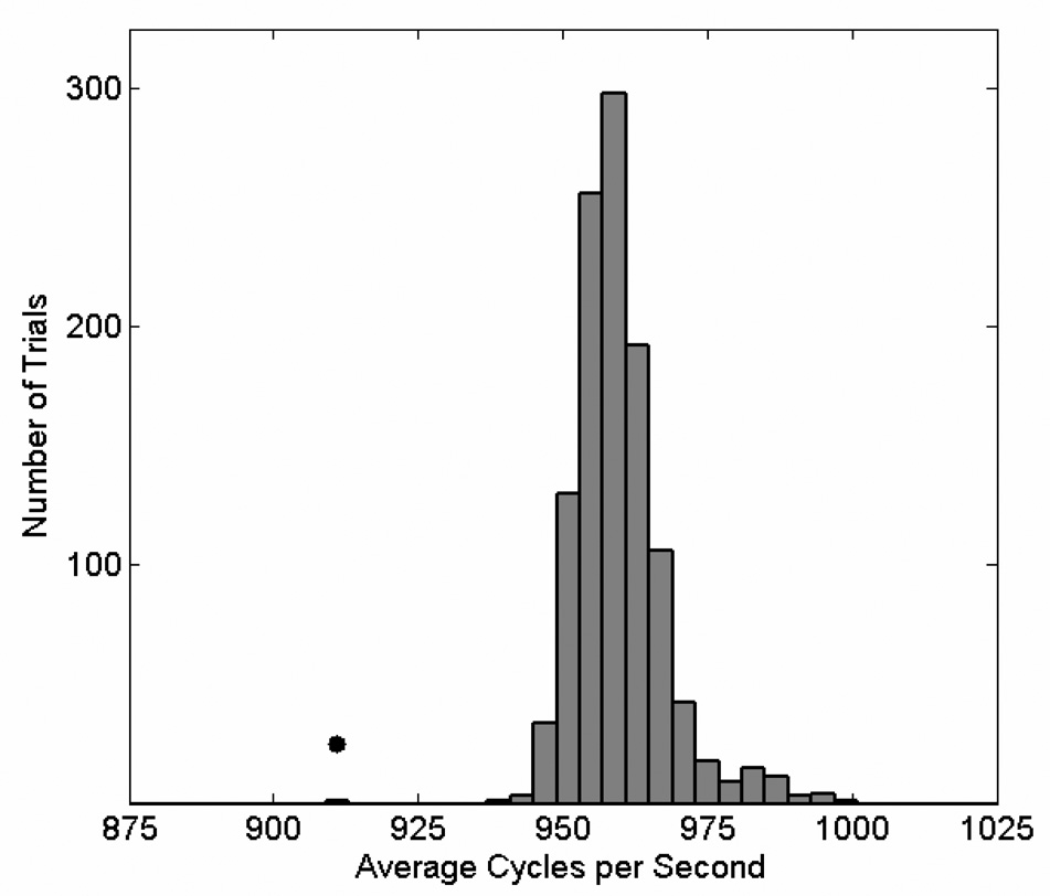
This histogram shows the mean cycle-rates for each trial over the behavioral session. As previously described (Asaad and Eskandar, 2008) the cycle rate of the first trial is typically lower, as marked here with a dot, representing 913 cycles per second. The next-slowest trial averaged 941 cycles per second. The mean cycle rate across all these trials except the first was 960. These rates include all cycles performed within the track function, including the first. Significantly faster cycle rates (> 2000 per second) have been observed on newer-generation PC systems. Note that only correct-choice and incorrect-choice trials are shown, because other trial types placed different demands on stimulus presentation and tracking (i.e., average cycle-rates for break-fixation trials tended to be slightly lower, as relatively less time was spent tracking than was spent updating the screen, and no-fixation trials were slightly faster for the opposite reason). Over all trials, the range of cycle rates varied from 800 to 1020 Hz except for 3 instances in which the subject broke fixation nearly instantaneously, resulting in average cycle rates between 700 and 800 Hz.

(a) The cycle times for a typical behavioral tracking epoch are plotted. The y-axis is truncated at 3 ms (the first cycle time here is 26.5 ms). Note the periodically increased times corresponding to the 100 ms interval between updates to the behavioral trace in the experimenter’s display. (b) The distribution of individual cycle times across all epochs of behavioral tracking in 1600 trials (the entire first trial, and the first cycle in each tracking epoch of all subsequent trials, were excluded). Cycle time is plotted against the number of cycles on a logarithmic scale. Cycle times in the higher mode (above 1.5 milliseconds) were found to correspond exclusively to those cycles during which the eye-trace on the experimenter’s display was updated. (c) The relative distribution of high-latency events during behavioral tracking is shown. This histogram was triggered on the occurrence of behavioral tracking cycle times greater than 1.5 ms (here at time 0). The lighter shaded region at the top of each bar represents the area of the mean value +/− the standard deviation. The cycles immediately following the high-latency instances tended to be slightly increased in time (increased relative to baseline by 11.6%, or 0.11 ms). The minimum interval in any trial between two high latencies, each greater than 1.5 ms, was found to be 81 cycles. (d) A scatter diagram plotting the time for each cycle against the time for the subsequent one (excluding the first cycle in each tracking epoch). Multiple modes are more clearly visible in this plot, but the relative numbers within each cluster are more difficult to ascertain than in 3a because of density saturation. Mode 1 contained 99.0% of all points, corresponding to a typical tracking cycle. Mode 2 corresponded to the second cycle within each tracking period. Modes 3 and 4 corresponded to those cycles in which a screen update request was made. No clear pattern of occurrence distinguished these last two modes.

(a) The cycle times for a typical behavioral tracking epoch are plotted. The y-axis is truncated at 3 ms (the first cycle time here is 26.5 ms). Note the periodically increased times corresponding to the 100 ms interval between updates to the behavioral trace in the experimenter’s display. (b) The distribution of individual cycle times across all epochs of behavioral tracking in 1600 trials (the entire first trial, and the first cycle in each tracking epoch of all subsequent trials, were excluded). Cycle time is plotted against the number of cycles on a logarithmic scale. Cycle times in the higher mode (above 1.5 milliseconds) were found to correspond exclusively to those cycles during which the eye-trace on the experimenter’s display was updated. (c) The relative distribution of high-latency events during behavioral tracking is shown. This histogram was triggered on the occurrence of behavioral tracking cycle times greater than 1.5 ms (here at time 0). The lighter shaded region at the top of each bar represents the area of the mean value +/− the standard deviation. The cycles immediately following the high-latency instances tended to be slightly increased in time (increased relative to baseline by 11.6%, or 0.11 ms). The minimum interval in any trial between two high latencies, each greater than 1.5 ms, was found to be 81 cycles. (d) A scatter diagram plotting the time for each cycle against the time for the subsequent one (excluding the first cycle in each tracking epoch). Multiple modes are more clearly visible in this plot, but the relative numbers within each cluster are more difficult to ascertain than in 3a because of density saturation. Mode 1 contained 99.0% of all points, corresponding to a typical tracking cycle. Mode 2 corresponded to the second cycle within each tracking period. Modes 3 and 4 corresponded to those cycles in which a screen update request was made. No clear pattern of occurrence distinguished these last two modes.

(a) The cycle times for a typical behavioral tracking epoch are plotted. The y-axis is truncated at 3 ms (the first cycle time here is 26.5 ms). Note the periodically increased times corresponding to the 100 ms interval between updates to the behavioral trace in the experimenter’s display. (b) The distribution of individual cycle times across all epochs of behavioral tracking in 1600 trials (the entire first trial, and the first cycle in each tracking epoch of all subsequent trials, were excluded). Cycle time is plotted against the number of cycles on a logarithmic scale. Cycle times in the higher mode (above 1.5 milliseconds) were found to correspond exclusively to those cycles during which the eye-trace on the experimenter’s display was updated. (c) The relative distribution of high-latency events during behavioral tracking is shown. This histogram was triggered on the occurrence of behavioral tracking cycle times greater than 1.5 ms (here at time 0). The lighter shaded region at the top of each bar represents the area of the mean value +/− the standard deviation. The cycles immediately following the high-latency instances tended to be slightly increased in time (increased relative to baseline by 11.6%, or 0.11 ms). The minimum interval in any trial between two high latencies, each greater than 1.5 ms, was found to be 81 cycles. (d) A scatter diagram plotting the time for each cycle against the time for the subsequent one (excluding the first cycle in each tracking epoch). Multiple modes are more clearly visible in this plot, but the relative numbers within each cluster are more difficult to ascertain than in 3a because of density saturation. Mode 1 contained 99.0% of all points, corresponding to a typical tracking cycle. Mode 2 corresponded to the second cycle within each tracking period. Modes 3 and 4 corresponded to those cycles in which a screen update request was made. No clear pattern of occurrence distinguished these last two modes.

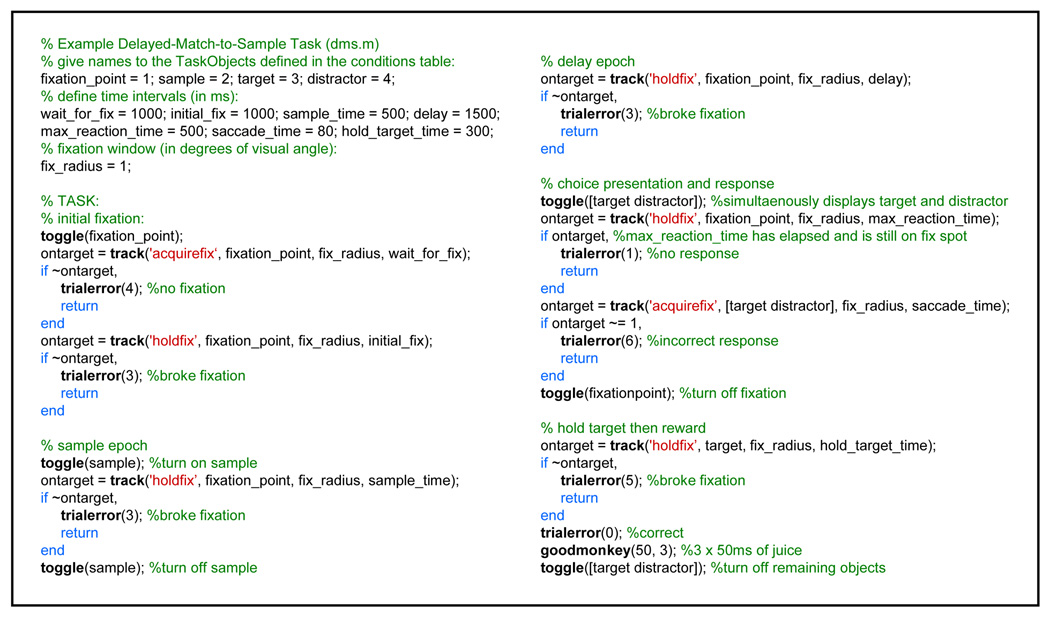
The over-all task design of a standard DMS task is shown in (a). The task consists of a fixation period, sample period, delay period, and then the presentation of choices. The subject’s goal is to select that object among the choices that matches the sample cue, by making a saccade to that object. The subject must fixate on the central dot throughout the task until the choices are presented. (b) A conditions table describing this task. This table allows for either of two pairs of objects to be used on any given trial: pictures A & B, or pictures C & D. “Relative Frequency” determines how likely a particular condition is to be chosen, relative to the other conditions. “Conditions in Block” enumerates the blocks in which that particular condition can appear (for instance, running block #2 would play only conditions 5–8, and so would use only pictures C & D). “Timing File” refers to the Matlab script that organizes the contingencies that relate behavioral monitoring to stimulus presentation (as in (c), below). Here, all conditions use the same timing file. “Object” columns list the stimuli that can appear in each condition. These can be visual objects, sounds, analog waveforms, or TTL pulses; any type of stimulus object can be triggered with the same toggle command. Note that, to simplify coding of the timing script, objects serving the same purpose are always in the same column (so, here, the sample object is always Object #2 and the target is always #3). (c) The Matlab script constituting the timing file used for this DMS task is shown. Functions that are provided by our software are highlighted in bold. Several other functions exist for time-stamping behaviorally-relevant events, repositioning-objects on-the-fly, turning the joystick-cursor on and off, defining interactive “hot keys” that initiate user-defined functions when the a key is pressed, etc.

The over-all task design of a standard DMS task is shown in (a). The task consists of a fixation period, sample period, delay period, and then the presentation of choices. The subject’s goal is to select that object among the choices that matches the sample cue, by making a saccade to that object. The subject must fixate on the central dot throughout the task until the choices are presented. (b) A conditions table describing this task. This table allows for either of two pairs of objects to be used on any given trial: pictures A & B, or pictures C & D. “Relative Frequency” determines how likely a particular condition is to be chosen, relative to the other conditions. “Conditions in Block” enumerates the blocks in which that particular condition can appear (for instance, running block #2 would play only conditions 5–8, and so would use only pictures C & D). “Timing File” refers to the Matlab script that organizes the contingencies that relate behavioral monitoring to stimulus presentation (as in (c), below). Here, all conditions use the same timing file. “Object” columns list the stimuli that can appear in each condition. These can be visual objects, sounds, analog waveforms, or TTL pulses; any type of stimulus object can be triggered with the same toggle command. Note that, to simplify coding of the timing script, objects serving the same purpose are always in the same column (so, here, the sample object is always Object #2 and the target is always #3). (c) The Matlab script constituting the timing file used for this DMS task is shown. Functions that are provided by our software are highlighted in bold. Several other functions exist for time-stamping behaviorally-relevant events, repositioning-objects on-the-fly, turning the joystick-cursor on and off, defining interactive “hot keys” that initiate user-defined functions when the a key is pressed, etc.
The over-all task design of a standard DMS task is shown in (a). The task consists of a fixation period, sample period, delay period, and then the presentation of choices. The subject’s goal is to select that object among the choices that matches the sample cue, by making a saccade to that object. The subject must fixate on the central dot throughout the task until the choices are presented. (b) A conditions table describing this task. This table allows for either of two pairs of objects to be used on any given trial: pictures A & B, or pictures C & D. “Relative Frequency” determines how likely a particular condition is to be chosen, relative to the other conditions. “Conditions in Block” enumerates the blocks in which that particular condition can appear (for instance, running block #2 would play only conditions 5–8, and so would use only pictures C & D). “Timing File” refers to the Matlab script that organizes the contingencies that relate behavioral monitoring to stimulus presentation (as in (c), below). Here, all conditions use the same timing file. “Object” columns list the stimuli that can appear in each condition. These can be visual objects, sounds, analog waveforms, or TTL pulses; any type of stimulus object can be triggered with the same toggle command. Note that, to simplify coding of the timing script, objects serving the same purpose are always in the same column (so, here, the sample object is always Object #2 and the target is always #3). (c) The Matlab script constituting the timing file used for this DMS task is shown. Functions that are provided by our software are highlighted in bold. Several other functions exist for time-stamping behaviorally-relevant events, repositioning-objects on-the-fly, turning the joystick-cursor on and off, defining interactive “hot keys” that initiate user-defined functions when the a key is pressed, etc.

A basic overview of performance is shown in (a). Behavior over time is plotted at the top, reaction times are shown at the bottom-right, and basic file information and trial-selection is at the bottom-left. In the bottom-middle is an area which shows the objects used on the currently-selected trial and the eye- or joystick record. The trial can be played back in this window by pressing “Play,” and a movie can be created from any trial. (b) A time-line representation of the currently-selected trial. X- and Y-eye or joystick traces are shown at the bottom. The horizontal red bars indicate that the object at left was currently visible. The vertical green lines indicate reward delivery (here, three pulses of juice).

A basic overview of performance is shown in (a). Behavior over time is plotted at the top, reaction times are shown at the bottom-right, and basic file information and trial-selection is at the bottom-left. In the bottom-middle is an area which shows the objects used on the currently-selected trial and the eye- or joystick record. The trial can be played back in this window by pressing “Play,” and a movie can be created from any trial. (b) A time-line representation of the currently-selected trial. X- and Y-eye or joystick traces are shown at the bottom. The horizontal red bars indicate that the object at left was currently visible. The vertical green lines indicate reward delivery (here, three pulses of juice).
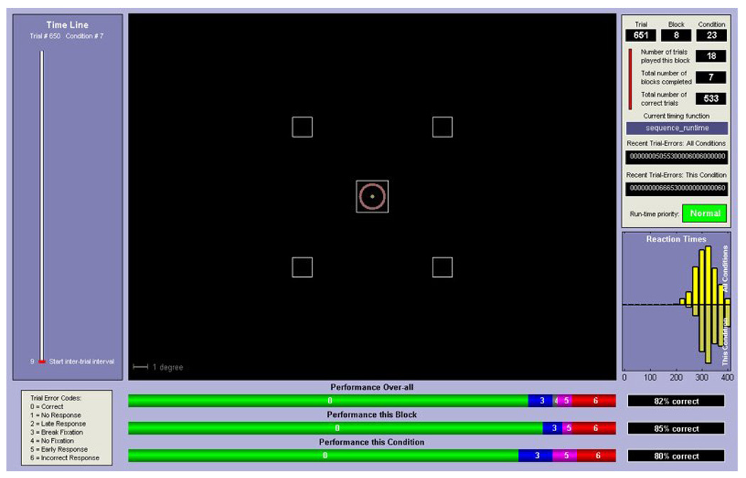
The experimenter’s display (a) contains a representation of the stimuli currently visible on the subject’s display (b). In addition, a red ring marks the boundaries of the current fixation (or joystick target) window and a dot represents the current eye- or joystick-position (updates are generally set to occur every 50 or 100 ms, depending on user preferences). In the top-right, the experimenter’s display relays information about the current trial, condition, block numbers and performance over-all, over the current block, and for the current condition. Reaction time histograms over-all and for the current condition are plotted at the lower-right.

The experimenter’s display (a) contains a representation of the stimuli currently visible on the subject’s display (b). In addition, a red ring marks the boundaries of the current fixation (or joystick target) window and a dot represents the current eye- or joystick-position (updates are generally set to occur every 50 or 100 ms, depending on user preferences). In the top-right, the experimenter’s display relays information about the current trial, condition, block numbers and performance over-all, over the current block, and for the current condition. Reaction time histograms over-all and for the current condition are plotted at the lower-right.

This menu is where an experiment and all of its configuration parameters can be loaded, modified, and saved. Video settings are organized within the left panel. Input-output assignments and other settings are found within the right panel. Task-execution settings (e.g., condition- and block-selection criteria) are in the middle panel. This menu is the point from which an experiment is launched.
References
-
- Brainard DH. The Psychophysics Toolbox. Spat Vis. 1997;10:433–436. - PubMed
-
- Ghose GM, Ohzawa I, Freeman RD. A flexible PC-based physiological monitor for animal experiments. J Neurosci Methods. 1995;62:7–13. - PubMed
-
- Hays AV, Richmond BJ, Optican LM. A UNIX-based multiple-process system for real-time data acquisition and control; WESCON Conference Proceedings; 1982. pp. 1–10.
-
- Judge SJ, Wurtz RH, Richmond BJ. Vision during saccadic eye movements. I. Visual interactions in striate cortex. Journal of Neurophysiology. 1980;43:1133–1155. - PubMed
Publication types
MeSH terms
Grants and funding
LinkOut - more resources
Full Text Sources
Other Literature Sources
