Kriging and Semivariogram Deconvolution in the Presence of Irregular Geographical Units

Abstract

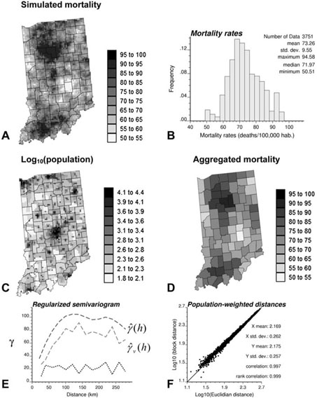
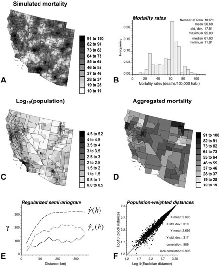
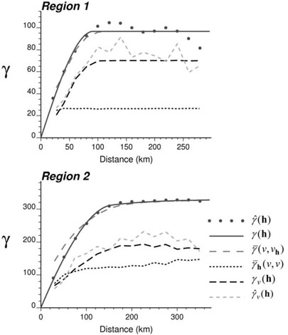
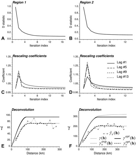
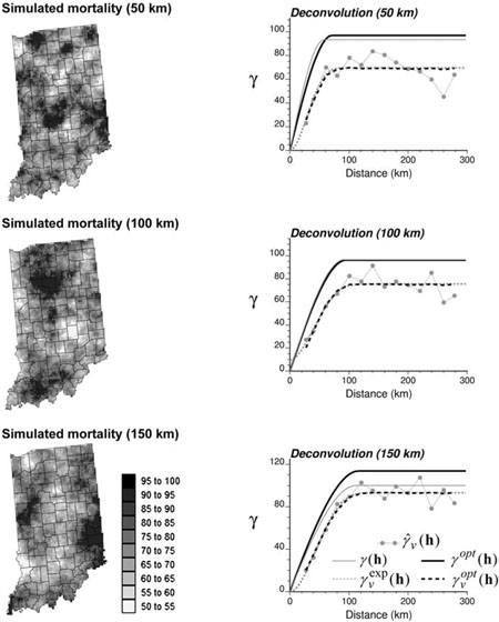
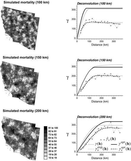
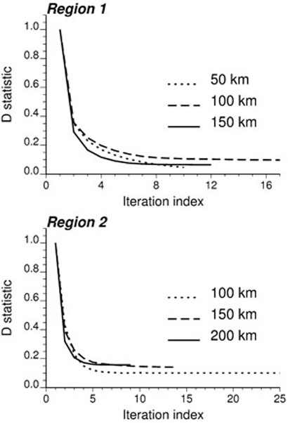
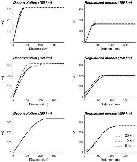
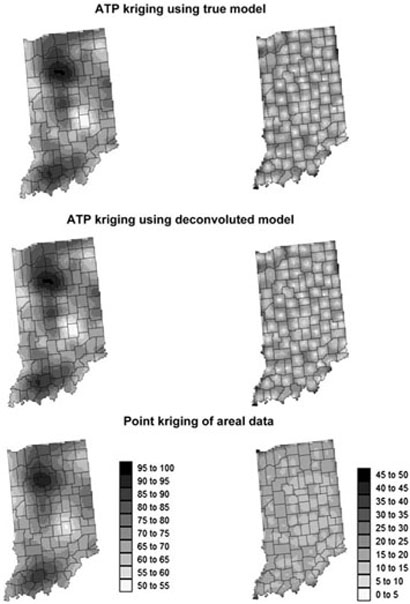
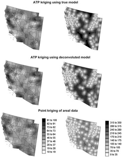
This paper presents a methodology to conduct geostatistical variography and interpolation on areal data measured over geographical units (or blocks) with different sizes and shapes, while accounting for heterogeneous weight or kernel functions within those units. The deconvolution method is iterative and seeks the pointsupport model that minimizes the difference between the theoretically regularized semivariogram model and the model fitted to areal data. This model is then used in area-to-point (ATP) kriging to map the spatial distribution of the attribute of interest within each geographical unit. The coherence constraint ensures that the weighted average of kriged estimates equals the areal datum.This approach is illustrated using health data (cancer rates aggregated at the county level) and population density surface as a kernel function. Simulations are conducted over two regions with contrasting county geographies: the state of Indiana and four states in the Western United States. In both regions, the deconvolution approach yields a point support semivariogram model that is reasonably close to the semivariogram of simulated point values. The use of this model in ATP kriging yields a more accurate prediction than a naïve point kriging of areal data that simply collapses each county into its geographic centroid. ATP kriging reduces the smoothing effect and is robust with respect to small differences in the point support semivariogram model. Important features of the point-support semivariogram, such as the nugget effect, can never be fully validated from areal data. The user may want to narrow down the set of solutions based on his knowledge of the phenomenon (e.g., set the nugget effect to zero). The approach presented avoids the visual bias associated with the interpretation of choropleth maps and should facilitate the analysis of relationships between variables measured over different spatial supports.

Fig. 1

(A) Simulated mortality map (5 km resolution) in Indiana (Region 1). (B)Mortality rates in Indiana (Region 1). Accounting for the population density (C), mortality values are aggregated within each of the 92 counties (D). Bottom graph shows the omnidirectional semivariograms of mortality before ŷ(h)) and after (ŷ_ν(h)) aggregation, and their difference (E). The scattergram plots Euclidean distances between county centroids versus a “block distance” that accounts for the shape of counties and the distribution of the population (F).

Fig. 2

(A) Simulated mortality map (5 km resolution) in four states of the Western US (Region 2). (B) Mortality rates in western US. Accounting for the population density (C), mortality values are aggregated within each of the 118 counties (D). Bottom graph shows the omnidirectional semivariograms of mortality before (ŷ(h)) and after (ŷ_ν(h)) aggregation, and their difference (E). The scattergram plots Euclidean distances between county centroids versus a ‘block distance’ that accounts for the shape of counties and the distribution of the population (F).

Fig. 3

Application of the regularization equation (21) to the point support semivariogram model γ(h) fitted to experimental values (black dots) for Regions 1 and 2. The theoretically regularized semivariogram model γ_ν(h), computed as the difference ${\gamma }_{\nu }(\mathbf{\text{h}})=\overline{\gamma }(\nu ,{\nu }_{\mathbf{\text{h}}})-{\overline{\gamma }}_{\mathbf{\text{h}}}(\nu ,\nu )$, is compared to the experimental semivariogram ${\widehat{\gamma }}_{\nu }(\mathbf{\text{h}})$ computed directly from areal data.

Fig. 4

Application of the deconvolution procedure to the regularized semivariograms of Regions 1 and 2. As the iteration progresses, the lag-specific rescaling coefficients (C, D) converge to one while the D statistic (A, B), which measures the difference between the theoretically regularized model ${\gamma }_{\nu }^{\text{opt}}(\mathbf{\text{h}})$ and the experimental curve ${\gamma }_{\nu }^{\text{exp}}(\mathbf{\text{h}})$, declines. In both regions (E, F) the deconvoluted model γ^opt(h) is reasonably close to the “true” point support model γ (h).

Fig. 5

Mortality simulated in Region 1 using three spherical models with no nugget effect and increasing ranges. Right column shows the results of the deconvolution. In all cases, the deconvoluted model γ^opt(h) is reasonably close to the “true” point support model γ (h). The similarity of the theoretically regularized model ${\gamma }_{\nu }^{\text{opt}}(\mathbf{\text{h}})$ and the experimental curve ${\gamma }_{\nu }^{\text{exp}}(\mathbf{\text{h}})$ illustrates the ability of the iterative procedure to achieve a solution.

Fig. 6

Mortality simulated in Region 2 using three spherical models with no nugget effect and increasing ranges. Right column shows the results of the deconvolution. In all cases, the deconvoluted model γ^opt(h) is reasonably close to the “true” point support model γ (h). The similarity of the theoretically regularized model ${\gamma }_{\nu }^{\text{opt}}(\mathbf{\text{h}})$ and the experimental curve ${\gamma }_{\nu }^{\text{exp}}(\mathbf{\text{h}})$ illustrates the ability of the iterative procedure to achieve a solution.

Fig. 7

Evolution of the D statistic during the iterative procedure of deconvolution for three different spatial patterns (spherical semivariogram models with increasing range) in Regions 1 and 2.

Fig. 8

Impact of the spatial resolution of the discretizing grid (i.e., 5, 10, or 20 km spacing grid) on the model fitted to the semivariogram of areal data (right column) and the results of the deconvolution (left column). The analysis was conducted for the three simulated maps of Region 2, using ranges of autocorrelation equal to 100, 150, and 200 km.

Fig. 9

Maps of kriging estimates (left) and variances (right) computed for the 100 km range spatial pattern in Region 1 using three alternative interpolation methods: ATP kriging using true point support model γ(h), ATP kriging using deconvoluted model, and point kriging of areal data.

Fig. 10

Maps of kriging estimates (left) and variances (right) computed for the 150 km range spatial pattern in Region 2 using three alternative interpolation methods: ATP kriging using true point support model γ(h), ATP kriging using deconvoluted model, and point kriging of areal data.

References

-
- Armstrong M. Basic linear geostatistics. Springer, Berlin: 1998. p. 172.
- Barabás N, Goovaerts P, Adriaens P. Geostatistical assessment and validation of uncertainty for three-dimensional dioxin data from sediments in an estuarine river. Environ Sci Technol. 2001;35(16):3294–3301. - PubMed
- Chiles JP, Delfiner P. Geostatistics: modeling spatial uncertainty. Wiley, New York: 1999. p. 720.
Grants and funding
LinkOut - more resources
Full Text Sources