. 2008 Sep 10;28(37):9151-63.
doi: 10.1523/JNEUROSCI.1789-08.2008.

Linking the response properties of cells in auditory cortex with network architecture: cotuning versus lateral inhibition

Affiliations

Linking the response properties of cells in auditory cortex with network architecture: cotuning versus lateral inhibition

Jaime de la Rocha et al. J Neurosci. .

Abstract

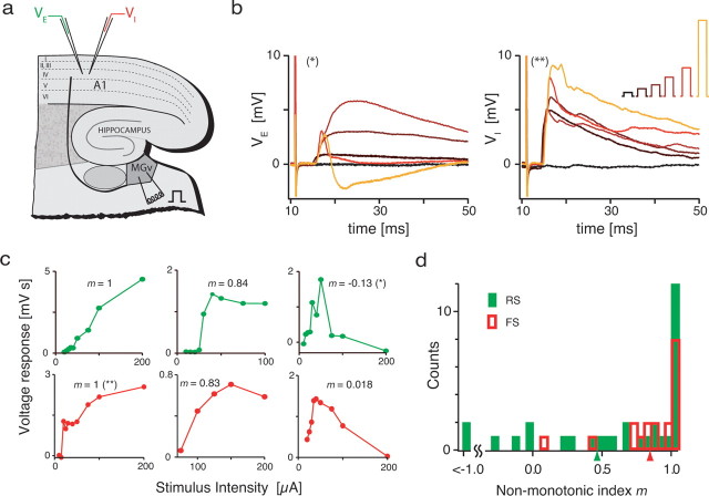
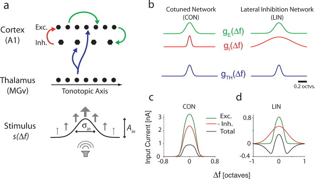
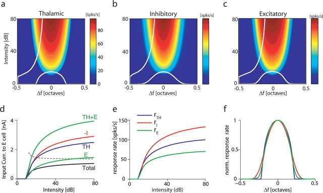
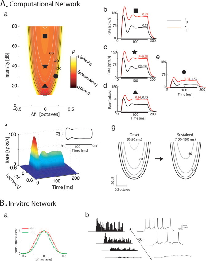
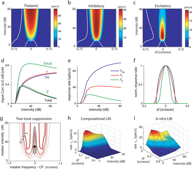
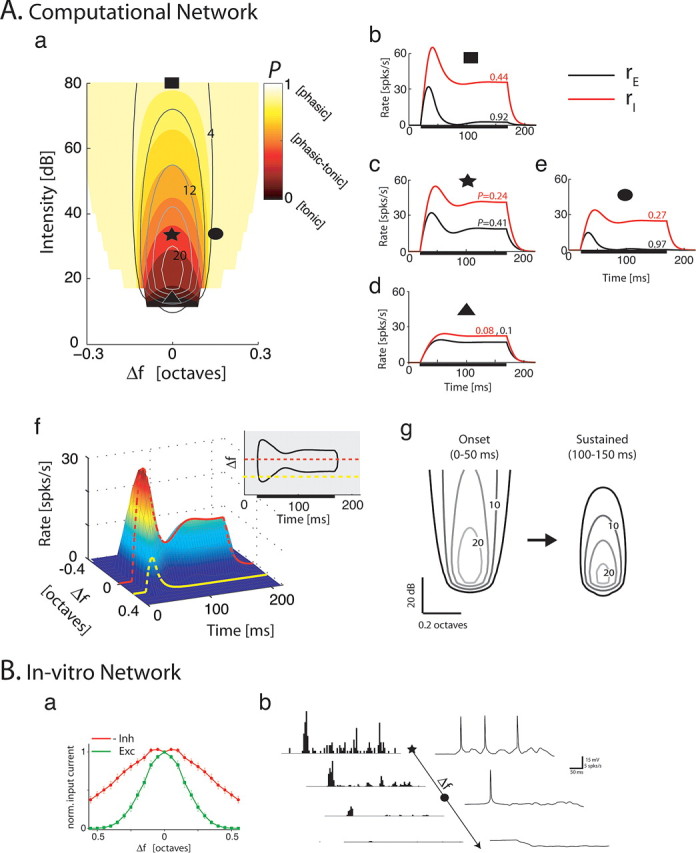
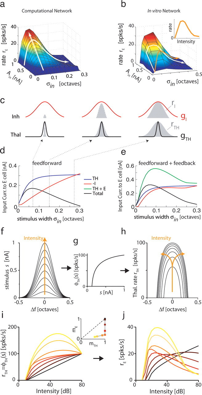
The frequency-intensity receptive fields (RF) of neurons in primary auditory cortex (AI) are heterogeneous. Some neurons have V-shaped RFs, whereas others have enclosed ovoid RFs. Moreover, there is a wide range of temporal response profiles ranging from phasic to tonic firing. The mechanisms underlying this diversity of receptive field properties are yet unknown. Here we study the characteristics of thalamocortical (TC) and intracortical connectivity that give rise to the individual cell responses. Using a mouse auditory TC slice preparation, we found that the amplitude of synaptic responses in AI varies non-monotonically with the intensity of the stimulation in the medial geniculate nucleus (MGv). We constructed a network model of MGv and AI that was simulated using either rate model cells or in vitro neurons through an iterative procedure that used the recorded neural responses to reconstruct network activity. We compared the receptive fields and firing profiles obtained with networks configured to have either cotuned excitatory and inhibitory inputs or relatively broad, lateral inhibitory inputs. Each of these networks yielded distinct response properties consistent with those documented in vivo with natural stimuli. The cotuned network produced V-shaped RFs, phasic-tonic firing profiles, and predominantly monotonic rate-level functions. The lateral inhibitory network produced enclosed RFs with narrow frequency tuning, a variety of firing profiles, and robust non-monotonic rate-level functions. We conclude that both types of circuits must be present to account for the wide variety of responses observed in vivo.


Figures

Figure 1.
Figure 1.
Postsynaptic potentials evoked with thalamic stimulation. a, Schematic of thalamocortical auditory slice preparation. Brief stimulus pulses (200 μs) were delivered to MGv and the PSPs recorded simultaneously in RS and FS cells in layer 4. b, PSPs (averaged from 10–15 trials) evoked at different stimulus intensities (10, 20, 30, 50, 75, and 200 μA; see inset color code) from an RS (left) and an FS (right) cell, simultaneously recorded. Action potentials were digitally filtered from voltage traces (see Materials and Methods). c, PSP area (calculated over a window of 50 ms from PSP onset) versus stimulus intensity for three RS cells (top row) and three FS cells (bottom row). Some cells (middle and right columns) showed distinct non-monotonic curves. Cells indicated with * and ** were those shown in a. d, Population histogram of the non-monotonicity index m (Eq. 12), defined as the ratio of the response at maximum intensity to the maximum response. A larger fraction of RS cells (green) displayed non-monotonic behavior (15 of 33 RS vs 4 of 19 FS cells showed m < 0.75) and overall had a lower mean m (0.46 for RS vs 0.84 for FS; triangles).
Figure 2.
Figure 2.
Implementation of cotuned and lateral inhibitory networks. a, Schematic of the thalamocortical network model. Cells in the TH and cortical layers are spatially arranged along a tonotopic axis. The cortical layer is composed of E and I cells. TC afferents formed connections with E and I cells (blue arrows), I cells were connected to E cells (red), and E cells are connected to E and I cells (green). Inputs to thalamus during the presentation of a tone were modeled as a Gaussian distributed current sf) with amplitude Ain and width σin. b, CON and LIN are defined by connectivity functions, gαf) (α = TH, E, I; color code matched with a). In the LIN, the connectivity function for inhibition is wider than that for TC or the E, whereas in the CON it is slightly narrower. c, d, Synaptic currents generated in a reference E cell in the cortical layer. In the CON, the excitation and inhibition vary proportionally with increasing Δf, and the total current is approximately Gaussian (black in c). In the LIN, the tuning of inhibitory inputs is broader so that the total current has a Mexican hat shape (black in d).
Figure 3.
Figure 3.
Receptive field properties in the CON. a–c, RFs of TH, I, and E cells calculated by varying stimulus frequency and intensity. The rate-level function obtained at CF and the tuning curve at 40 dB are shown on the left (rotated) and bottom, respectively, of each panel. d, Input currents into a reference E cell show a proportional recruitment of excitation (green curves) and inhibition (red curve) with increasing intensity. The ratio between the excitatory input and the inhibitory input (dashed line) is approximately constant. e, f, Rate-level functions (e) and frequency tuning curves (f) show that cortical E and I cells mimic the behavior of TH cells. Intensity was 40 db (f) and f = CF (e). Legend in e also applies to f.
Figure 4.
Figure 4.
Response dynamics in the CON. A, Computational network. a, Map of P index (color) superimposed on RF of an E cell (contour lines). The P index (Eq. 11) quantifies the relative magnitude of the transient and sustained components of the response profile. Except at large Δf, the response is always phasic-tonic. Symbols represent responses highlighted in b–e. b–d, Responses produced by tones at CF and high, moderate, and low intensity (■, ★, and ▲ in a, respectively) are approximately scaled versions of the same phasic-tonic pattern in E cells [rE(t), black]. The responses of the I cells [rI(t), red] were more tonic with a weak phasic component (see P values by the curves). The thick horizontal line in all plots shows the tone presentation interval. e, Increasing Δf (● in a) decreases both rE(t) and rI(t) with little variation of the pattern. f, Response pattern of the entire E population to a 40 dB tone. Inset shows the iso-rate contour line at half-maximum. g, Iso-rate contour lines of the RF of an E cell computed during the onset (interval, 0–50 ms) and sustained (interval, 100–150 ms) parts of the response. B, In vitro model network. a, Normalized average excitatory and inhibitory currents into an E cell show cotuning. b, PSTHs (left) and representative voltage traces (right) of an E cell as frequency deviates from CF. As in the computational model, increasing Δf scales down the entire response. Parameters in Aa–Ae are as follows: T = 150 ms; (Δf, I) = (0, 40) (★), (0,70) (■), (0,20) (▲), (0.4, 20) (●), all in octaves and decibels. Labels on contour lines in a indicate firing rate in spikes per second. Parameters in Ba, Bb are as follows: T = 360 ms; Δf = 0, 0.1, 0.2, and 0.3 octaves; PSTH bin size, 5 ms (b, left); Δf = 0, 0.2, and 0.35 octaves (b, right).
Figure 5.
Figure 5.
Receptive field properties in the LIN. a–c, Receptive fields of a TH (a), I (b), and E (c) cells as in Figure 3. The E cell has a non-monotonic rate-level function (white trace on ordinate) and a sharper frequency tuning (white trace on abscissa) than the TH and I cells. d, Input currents into a reference E cell show an unbalanced recruitment of excitation (green curves) and inhibition (red curve) with increasing intensity. e, Rate-level functions using tones at CF show strong (slight) non-monotonicity in E (I) cells. f, Frequency tuning curves at 40 dB show strong (moderate) sharpening in E (I) cells. g, Suppressive receptive field obtained by the simultaneous presentation of a fixed probe tone (star) and a masker tone that was systematically varied in frequency and intensity. Red curves indicate the areas in which the masker suppressed the probe response by the amount indicated in the labels. Shaded area shows the RF of the probe alone thresholded at half-height. Because of the recruitment of lateral inhibition by the masker, a prominent suppressive RF flanks the excitatory RF, forming a W shape. h, Surface plot of RF obtained with shorter tones (T = 100 ms) than in c (T = 150 ms). There was a reduction in the degree of non-monotonicity; tones away from CF produced monotonic functions. i, In vitro network. RF of an E cell obtained with the in vitro LIN with only feedforward connections. Legend in e also applies to f.
Figure 6.
Figure 6.
Response dynamics in the LIN. Legend as in Figure 4. A, Computational network. a, Map of P index (color) superimposed on RF of an E cell (contour lines). For f ∼ CF, increasing intensity causes the response to switch from tonic, to phasic-tonic, to phasic. Symbols represent responses highlighted in b–e. b–d, Responses of excitatory [rE(t), black] and inhibitory [rI(t), red] cells to a tone at CF and high (b), moderate (c), and low (d) intensity (■, ★, and ▲ in a, respectively). Numbers on the curves indicate P values. e, rE(t) and rI(t) for a stimulus of moderate intensity and Δf > 0 (● in a). f, Response pattern of the entire E population to a 30 dB tone. Inset shows the iso-rate contour line at half-maximum. g, Iso-rate contour lines of the RF of an E cell computed during the onset (interval, 0–50 ms) and sustained (interval, 100–150 ms) parts of the response. B, In vitro model network. a, Normalized average excitatory and inhibitory input currents versus Δf into a reference E cell show strong lateral inhibition. b, PSTHs (left) and representative voltage traces (right) of an E cell as frequency deviates from CF (top to bottom). Parameters in Aa–Ae: T = 130 ms; (Δf, I) = (0, 30) (★), (0,80) (■), (0,14) (▲), (0.15, 30) (•), all in octaves and decibels. Parameters in Ba, Bb: T = 360 ms; Δf = 0, 0.1, 0.2, and 0.3 octaves; PSTH bin size, 5 ms (b, left); Δf = 0, 0.2, and 0.35 octaves (b, right).
Figure 7.
Figure 7.
Unbalanced recruitment of excitation and inhibition in the LIN. a, Computational network. Surface plot of the response rate rE as a function of the amplitude Ain and spread of the thalamic input σin when using a threshold-linear thalamic transfer function φTH(s) (see Results). The response rE increases monotonically with Ain and non-monotonically with σin (white arrows). b, In vitro network. This result was reproduced using the in vitro LIN in which increasing intensity was modeled as either an ad hoc simultaneous increase in Ain and σin (orange track) or an increase in Ain followed by an increase in σin (white track). Both alternatives yield a non-monotonic rate–intensity function (inset). c, Thalamic population activity (rTHf), bottom shaded areas) and inhibitory population activity [rIf), top shaded areas] superimposed on the connectivity functions gTHf) (black) and gIf) (red) for three values of the stimulus spread. For details, see Results. d, Plot of individual currents generated in a reference E cell versus stimulus spread (examples in c correspond to those points indicated by dashed lines in d). e, Similar non-monotonic functions were obtained in an LIN network with intracortical feedback, although the individual currents behaved differently (see Results). f, Tone intensity was encoded in the amplitude Ain (at a fixed σin) of the stimulus function (Eq. 4). g, Using a nonlinear concave thalamic response function φTH(s) causes the amplitude and spread of the thalamic activity to increase with intensity (h). i, j, Decreasing the degree of concavity of φTH(s) reduces the degree of non-monotonicity of the rate-level function. A monotonic function is obtained when φTH(s) becomes linear (black). Making φTH(s) slightly non-monotonic sharpened the intensity tuning in cortex (yellow curves). This sharpening is summarized in the mTHmE mapping shown in the inset. Parameters in c–e: Ain = 0.5 nA; f–h: intensity varies from 0 to 80 dB in 10 dB steps; i, j: concavity varies from yellow to brown (b, c) = (4,0.2), (2.7,0.2), (1,0.2), (0,0.5), (0,0.1), (0,0.02), (0,0.001) and linear; c = 0.2 in the rest; f = CF.

Similar articles

Cited by

References

    1. Abeles M, Goldstein MH., Jr Responses of single units in the primary auditory cortex of the cat to tones and to tone pairs. Brain Res. 1972;42:337–352. - PubMed
    1. Aitkin LM, Webster WR. Medial geniculate body of the cat: organization and responses to tonal stimuli of neurons in ventral division. J Neurophysiol. 1972;35:365–380. - PubMed
    1. Atencio CA, Schreiner CE. Spectrotemporal processing differences between auditory cortical fast-spiking and regular-spiking neurons. J Neurosci. 2008;28:3897–3910. - PMC - PubMed
    1. Atzori M, Lei S, Evans DI, Kanold PO, Phillips-Tansey E, McIntyre O, McBain CJ. Differential synaptic processing separates stationary from transient inputs to the auditory cortex. Nat Neurosci. 2001;4:1230–1237. - PubMed
    1. Ben-Yishai R, Bar-Or RL, Sompolinsky H. Theory of orientation tuning in visual cortex. Proc Natl Acad Sci U S A. 1995;92:3844–3848. - PMC - PubMed

Publication types

MeSH terms

LinkOut - more resources