Parametric study of EEG sensitivity to phase noise during face processing

Abstract

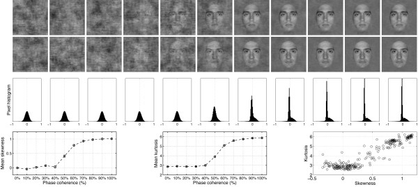
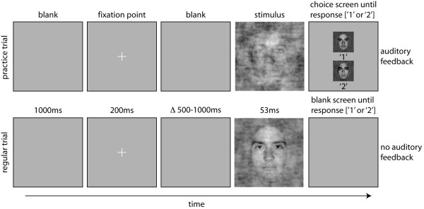
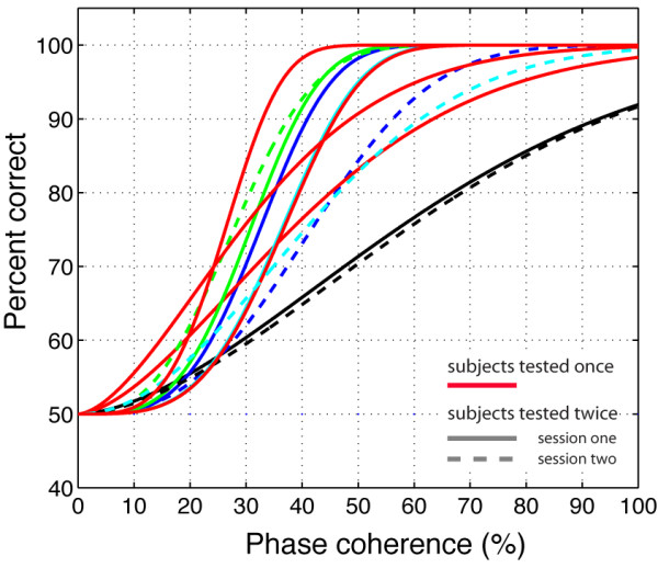
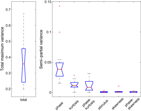
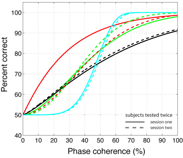
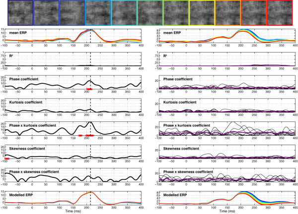
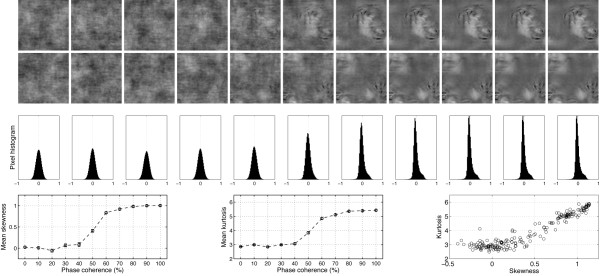
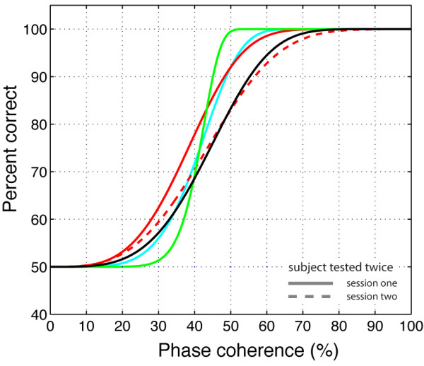
Background: The present paper examines the visual processing speed of complex objects, here faces, by mapping the relationship between object physical properties and single-trial brain responses. Measuring visual processing speed is challenging because uncontrolled physical differences that co-vary with object categories might affect brain measurements, thus biasing our speed estimates. Recently, we demonstrated that early event-related potential (ERP) differences between faces and objects are preserved even when images differ only in phase information, and amplitude spectra are equated across image categories. Here, we use a parametric design to study how early ERP to faces are shaped by phase information. Subjects performed a two-alternative force choice discrimination between two faces (Experiment 1) or textures (two control experiments). All stimuli had the same amplitude spectrum and were presented at 11 phase noise levels, varying from 0% to 100% in 10% increments, using a linear phase interpolation technique. Single-trial ERP data from each subject were analysed using a multiple linear regression model.

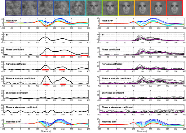
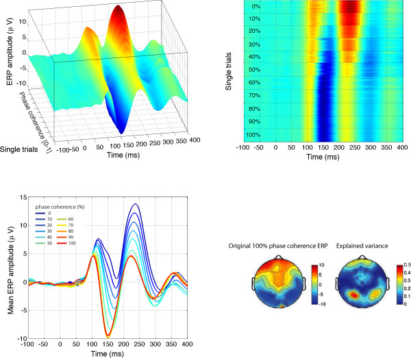
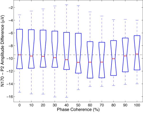
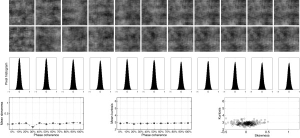
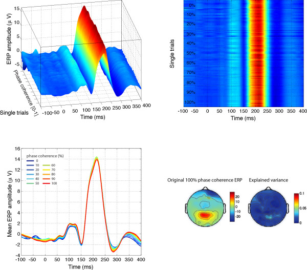
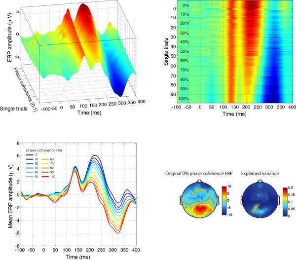
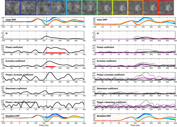
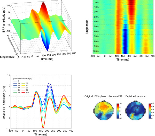
Results: Our results show that sensitivity to phase noise in faces emerges progressively in a short time window between the P1 and the N170 ERP visual components. The sensitivity to phase noise starts at about 120-130 ms after stimulus onset and continues for another 25-40 ms. This result was robust both within and across subjects. A control experiment using pink noise textures, which had the same second-order statistics as the faces used in Experiment 1, demonstrated that the sensitivity to phase noise observed for faces cannot be explained by the presence of global image structure alone. A second control experiment used wavelet textures that were matched to the face stimuli in terms of second- and higher-order image statistics. Results from this experiment suggest that higher-order statistics of faces are necessary but not sufficient to obtain the sensitivity to phase noise function observed in response to faces.

Conclusion: Our results constitute the first quantitative assessment of the time course of phase information processing by the human visual brain. We interpret our results in a framework that focuses on image statistics and single-trial analyses.

Figure 1

Examples of stimuli used in Experiment 1. The first two rows show the 22 stimuli presented to one observer during the first block of the experiment. The observer discriminated the same two faces during the whole experiment. The noise level varied from 100% (left side; 0% phase coherence) to 0% (right side; 100% phase coherence). Note that at each level of phase coherence the structure of the noise that was mixed with the original image was different, so that the task could not be performed based on the spatial characteristics of the noise. Histograms in the third row show the distribution of pixel contrasts averaged across all stimuli seen by this observer at each level of phase coherence. Starting with a Gaussian distribution (left), the pixel histograms become increasingly skewed and kurtotic with increasing phase coherence (right – the y-axes on the histograms are all the same). This relationship is depicted in the last row, showing the mean skewness (left), and mean kurtosis (middle), as a function of phase coherence. The error bars correspond to 95% confidence interval computed using a bootstrap percentile technique (1000 resamples). In the bottom right end graph, kurtosis for each image (each circle) is expressed as a function of skewness. Although the two statistical descriptors are correlated, the relationship is not linear. As demonstrated below, EEG amplitude is more sensitive to the kurtosis of the image than its skewness.

Figure 2

Organisation of practice trials (top row) and regular experimental trials (bottom row) in all experiments. The stimuli are examples taken from the main experiment that used faces (Experiment 1). A trial started with a blank screen for 1000 ms, followed by the presentation of a fixation point for 200 ms. Then, after a random delay ranging from 500 to 1000 ms, a stimulus was presented for 53 ms. During practice trials, a choice screen appeared immediately after the stimulus, showing the two targets of the experiment and their associated response keys. The screen stayed on until the subject's response, which was followed by auditory feedback, before the trial sequence resumed. During regular trials, a blank screen appeared immediately after the stimulus, and remained on until the subject's response. No feedback was provided during regular trials. Note that stimuli are not drawn to scale.

Figure 3

Percent correct for individual subjects in Experiment 1. The black lines show data from subject RXL. Subject RXL was singled-out because he is the only subject that was tested in experiment 1 and the two control experiments. The other colours depict data from all other observers and sessions. Continuous lines indicate the first recording session, while dashed lines indicate the second session of subjects who were tested twice. Data from subjects who were tested only once are indicated in red. Data were fit using a cumulative Weibull function where the accuracy p was expressed as a function of the phase coherence c, the phase coherence α supporting 82% threshold performance, and β the slope of the curve: $p=1-0.5e^{-{(c/\alpha )}^{\beta }}$

Figure 4

Session 1 of subject RXL (left) and data averaged across subjects (right) in Experiment 1. The vertical line in the left column indicates the latency of maximum R² for the model, recorded at electrode E107 for RXL, an electrode halfway between T5 and O1. Electrode E107 is at the centre of the left red cluster in the topographic map of explained variance in Figure 5. At the top, the row of face stimuli shows the colour code used in the mean ERP and modelled ERP plots, from blue (0% phase coherence) to red (100% phase coherence). The time course of the coefficient for the different model parameters is depicted in black, with the horizontal red line showing periods of statistically significant fitting (p < .01, not corrected for multiple comparisons). In the right column, purple lines show the mean coefficient across subjects and the thin black lines data from individual subjects. The beta coefficients are expressed in terms of signal change in μV per unit of the predictor variable.

Figure 5

Modelled data and topographical maps from session 1 of subject RXL in Experiment 1. The upper part of the figure shows 3D (left) and 2D (right) representations of single trials, sorted by chronological order in which they were recorded during the experiment, independently for each bin of phase coherence. In the lower left corner, single-trial modelled data were averaged according to phase coherence level, and colour coded from blue (0%) to red (100%) following Figure 4 nomenclature. The data are from the electrode at which the maximum R² was obtained. The topographic maps show the interpolated ERP signal (left, in μV) and explained variance (right, in %) at the latency of maximum R² (148 ms). The electrode showing the best fit is at the centre of the lower left red cluster in the explained variance map. For this subject, the electrode showing the maximum N170 was over the right hemisphere. However, at this electrode, the pattern of model fit was virtually indistinguishable from the one showed here.

Figure 6

Boxplots of total maximum explained variance and semi-partial variance in Experiment 1. For each subplot, the red line indicates the median. The blue box extends from the upper to the lower quartile values. The whiskers show the most extreme points that are within 1.5 times the inter-quartile range. A red plus is an outlier. The notch in the blue box corresponds to a robust estimate of the median confidence interval. Non-overlapping notches indicate that medians differ with 95% confidence. Because of the scaling involved in the computation of the semi-partial variance, the sum of semi-partial variances across regressors is less than the total explained variance. The semi-partial variance calculation was performed at the electrode and time point of maximum R² peak for each subject.

Figure 7

Boxplot of the peak-to-peak differences between the N170 and the P2 measured on modelled data at different levels of stimulus phase coherence for all subjects and sessions in Experiment 1.

Figure 8

Examples of stimuli used in Experiment 2. The first two rows show the 22 stimuli presented to one observer during the first block of the experiment. The observer discriminated between the same two textures during the whole experiment. The noise level varied from 100% (left side; 0% phase coherence) to 0% (right side; 100% phase coherence). Histograms in the third row show the distribution of pixel contrasts averaged across all stimuli seen by this observer at each level of phase coherence. Note that, unlike the stimuli used in Experiment 1, the pixel histograms had a relatively constant Gaussian distribution across all levels of phase coherence. This constant histogram distribution is depicted in the last row, showing the mean skewness (left), and mean kurtosis (middle), as a function of phase coherence. The error bars correspond to 95% confidence interval computed using a bootstrap percentile technique (1000 resamples). In the bottom right end graph, kurtosis for each image (each circle) is expressed as a function of skewness. There was no relationship between the two statistical descriptors.

Figure 9

Percent correct for individual subjects in Experiment 2. The black lines show data from subject RXL. The other colours depict data from all other observers and sessions. Continuous lines indicate the first recording session, while dashed lines indicate the second recording session.

Figure 10

Session 1 of subject RXL (left) and data averaged across subjects (right) in Experiment 2. Figure caption details are otherwise identical to those of Figure 4.

Figure 11

Modelled data and topographical maps from session 1 of subject RXL in Experiment 2. The topographic maps show data at the latency of maximum R² (214 ms). Figure caption details are otherwise identical to those of Figure 5.

Figure 12

Third EEG session from subject GAR in Experiment 2. The topographic maps show data at the latency of maximum R² (242 ms). It appears that data from this subject were particularly sensitive to phase information, as shown by the gradient of amplitude responses in the modelled data. However, the largest amount of variance explained was relatively low (R² = 0.13). Moreover, during the time range 200–300 ms, when the model provided the best fit to the data, none of the regressors were associated significantly with the EEG signal. Only at about 350 ms, a few time points show a significant phase by kurtosis interaction, but in this latency range, the maximum R² = 0.05.

Figure 13

Examples of stimuli used in Experiment 3. The first two rows show the 22 stimuli presented to one observer during the first block of the experiment. The observer discriminated the same two wavelet textures during the whole experiment. The noise level varied from 100% (left side; 0% phase coherence) to 0% (right side; 100% phase coherence). Histograms in the third row show the distribution of pixel contrasts averaged across the entire set of stimuli seen by this observer at each level of phase coherence, from 0% (left) to 100% (right). Similarly to what was observed for faces in Experiment 1, and contrary to the pink noise textures used in Experiment 2, the pixel histograms showed a non-linear transition from a Gaussian distribution to a skewed and kurtotic distribution with increasing levels of phase coherence. This progression is depicted in the last row, showing the mean skewness (left), and mean kurtosis (middle), as a function of phase coherence. The error bars correspond to 95% confidence interval computed using a bootstrap percentile technique (1000 resamples). In the bottom right end graph, kurtosis for each image (each circle) is expressed as a function of skewness. Similarly to face stimuli, the two statistical descriptors are non-linearly related to one another.

Figure 14

Percent correct for individual subjects in Experiment 3. The black lines show data from subject RXL. The other colours depict data from all other observers and sessions. Continuous lines indicate the first recording session, while dashed lines indicate the second recording session.

Figure 15

Session 1 of subject RXL (left) and data averaged across subjects (right) in Experiment 3. Figure caption details are otherwise identical to those of Figure 4.

Figure 16

Modelled data and topographical maps from session 1 of subject RXL in Experiment 3. The topographic maps show data at the latency of maximum R² (168 ms). This subject showed the earliest and the strongest sensitivity to phase noise. However, sensitivity to phase noise only starts to emerge at about 150 ms after stimulus onset, compared to about 120 ms in Experiment 1. Figure caption details are otherwise identical to those of Figure 5.

References

1. Bullier J, Hupe JM, James AC, Girard P. The role of feedback connections in shaping the responses of visual cortical neurons. Prog Brain Res. 2001;134:193–204. - PubMed
1. Bullier J. Integrated model of visual processing. Brain Research Reviews. 2001;36(2–3):96–107. - PubMed
1. DiCarlo JJ, Cox DD. Untangling invariant object recognition. Trends Cogn Sci. 2007;11(8):333–41. - PubMed
1. Rust NC, Movshon JA. In praise of artifice. Nat Neurosci. 2005;8(12):1647–50. - PubMed
1. Felsen G, Dan Y. A natural approach to studying vision. Nat Neurosci. 2005;8(12):1643–6. - PubMed
Publication types
MeSH terms
LinkOut - more resources