A high-resolution computational atlas of the human hippocampus from postmortem magnetic resonance imaging at 9.4 T

Abstract

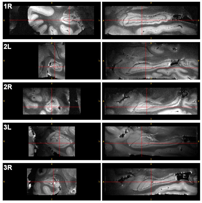
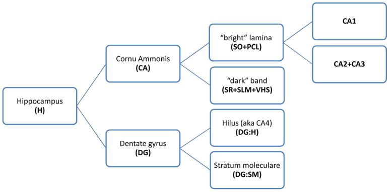
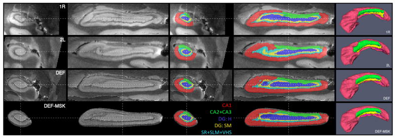
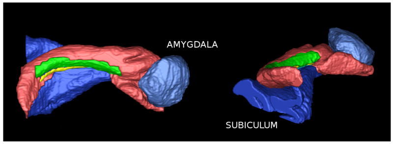
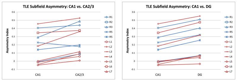
This paper describes the construction of a computational anatomical atlas of the human hippocampus. The atlas is derived from high-resolution 9.4 Tesla MRI of postmortem samples. The main subfields of the hippocampus (cornu ammonis fields CA1, CA2/3; the dentate gyrus; and the vestigial hippocampal sulcus) are labeled in the images manually using a combination of distinguishable image features and geometrical features. A synthetic average image is derived from the MRI of the samples using shape and intensity averaging in the diffeomorphic non-linear registration framework, and a consensus labeling of the template is generated. The agreement of the consensus labeling with manual labeling of each sample is measured, and the effect of aiding registration with landmarks and manually generated mask images is evaluated. The atlas is provided as an online resource with the aim of supporting subfield segmentation in emerging hippocampus imaging and image analysis techniques. An example application examining subfield-level hippocampal atrophy in temporal lobe epilepsy demonstrates the application of the atlas to in vivo studies.

Fig. 1

Coronal and sagittal slices through each of the hippocampus images included in the atlas. The acquisition parameters for these images are listed in Table 1. Image 3L has 0.2mm³ isotropic resolution; other images have resolution 0.3 × 0.2 × 0.3mm³.

Fig. 2

A diagram of the partitioning of the hippocampus into labels used in this paper. The abbreviations used in subsequent figures are in boldface. The leaf nodes in the graphs are the labels that were actually traced in the postmortem MR images. Later in the paper, segmentation repeatability and atlas consistency results are reported for the leaf nodes as well as for the parent-level structures formed by merging the labels corresponding to the leaf nodes. Abbreviations: SO = stratum oriens; PCL = pyramidal cell layer; SR = stratum radiatum; SLM = stratum lacunosum-moleculare; VHS = vestigial hippocampal sulcus.

Fig. 3

Coronal, sagittal and 3D views of hippocampus images and subfield labels for samples 1R and 2L, following aaffne alignment, and for atlases computed by unsupervised deformable registration (DEF) and mask-aided registration (DEF-MSK). Abbreviations: CA - cornu Ammonis; DG:H - hilus of the dentate gyrus (a.k.a. CA4); DG:SM - stratum moleculare of the dentate gyrus; SR - stratum radiatum; SLM - stratum lacunosum-moleculare; VHS -vestigial hippocampal sulcus.

Fig. 4

Hippocampus segmentation, along with the adjacent amygdala and subiculum (the subiculum label includes the presubiculum, the parasubiculum and parts of the parahippocampal cortex) Subfield color labels are the same as in Fig. 3.

Fig. 5

Analysis of segmentation repeatability, given in terms of Dice overlap between the full 3D segmentations used in constructing the atlas and repeated segmentations of a selected set of slices by two raters. Average Dice overlap for each subfield, as well as various combinations of subfields, is reported. See Fig. 2 for a diagram of the subfield labels appearing on the x-axis.

Fig. 6

Agreement between the consensus atlas labeling and segmentation of individual samples expressed in terms of average Dice overlap computed in atlas space. Six atlas-building approaches are compared: landmark-based and mask-based affne alignment (AFF-LM/AFF-MSK), image-based deformable normalization (DEF), deformable normalization aided by landmarks (DEF-LM), masks (DEF-MSK) and both masks and landmarks (DEF-LM-MSK). See Fig. 2 for a diagram of the subfield labels appearing on the x-axis.

Fig. 7

Agreement between the consensus atlas labeling and segmentation of individual samples expressed in terms of average distance between the boundaries of subfields in the atlas and the boundaries of corresponding subfields in warped individual segmentations. Refer to Fig. 6 for the explanation of different bars in the plot. See Fig. 2 for a diagram of the subfield labels appearing on the x-axis.

Fig. 8

Surface maps of root mean square distance between each subfield in the atlas and the corresponding subfield segmentation in each of the input images warped to the atlas. The atlas used in this figure was constructed using binary masks and no landmarks (DEF-MSK in Fig. 6). Larger values in the maps (yellow and red) indicate lesser coherence between the atlas and the individual segmentations. At the bottom left, all subfields in the atlas are shown together to provide a visual reference.

Fig. 9

A conceptual 2D illustration of shape-based normalization via the cm-rep coordinate system. The central curve is the skeleton m; the radial lines from the skeleton to the boundary are the spokes; the shape-based mapping between the two models is given by the locations of corresponding grid vertices.

Fig. 10

Illustration of cm-rep model fitting used for shape-based normalization. The top row shows the cm-rep model fitted to the “DEF-MSK” postmortem hippocampus atlas (see Fig. 3), and the other rows show models fitted to segmentations of the “healthy” hippocampus for three subjects in the TLE study (subjects L1, R2 and L4; selected arbitrarily). The left column shows the target structure, i.e., the segmentation of the hippocampus. The second column shows the skeleton surface m of the fitted cm-rep model, with the color map plotting the radius function R on the skeleton. The third column illustrates the spoke field; spokes are line segments extend from the skeleton to the boundary, are orthogonal to the boundary and “span” the interior of the model (see Fig. 9 for the 2D illustration of spokes). Spokes extending to boundary half b⁻ are shown in blue, and spokes that extend to b⁻ are shown in red. Correspondence on the basis of spoke fields is used to map subfield labels from the postmortem atlas to the in vivo data. The last column shows the boundary surface b = b⁺ ∪ b⁻, which closely approximates the surface of the target hippocampus.

Fig. 11

Example images from the in vivo temporal lobe epilepsy hippocampal asymmetry analysis experiment. Each row shows data from one of the subjects in the study. The first column shows a sagittal cross-section of the region surrounding the hippocampus contralateral to the seizure focus (“healthy” side). The second column shows the ipsilateral (“diseased”) hippocampus region after flipping across the midsagittal plane and rigid alignment to the healthy hippocampus. The third column plots the logarithm of the Jacobian of the transformation between the healthy hippocampus and diseased hippocampus computed by deformable image registration. Negative values (blue) indicate that a small region R in the healthy hippocampus maps to a smaller region in the diseased hippocampus; positive values (red) indicate the opposite. The Jacobian map is restricted to the the healthy hippocampus (i.e., to the manual segmentation). The last column shows the estimation of the location of hippocampal subfields in the healthy hippocampus. Subfields are mapped from the postmortem atlas using shape-based normalization.

Fig. 12

This figure plots the healthy/diseased asymmetry in TLE in a reference space, i.e., in the space of the postmortem hippocampus atlas. The left column shows 5 coronal slices and a sagittal slice through the postmortem atlas “DEF-MSK” (see Fig. 3), which is the atlas used in the TLE experiment. The second column shows the subfield labeling of the “DEF-MSK” atlas. The third column shows the logarithm of the Jacobian determinant of the mapping from the healthy hippocampus to the diseased hippocampus, averaged over all subjects. This average Jacobian map is computed by using shape-based normalization to transform the log-Jacobian maps shown in Fig. 11 back into atlas space, followed by computing the average. Negative values (blue) indicate local volumetric decrease (disease-associated atrophy); positive values (red) indicate local increase in volume. The last column shows corresponding slices from the non-masked postmortem atlas “DEF”, for the purpose of visualizing the adjacent tissues.

Fig. 13

Plots of volumetric asymmetry between the subfields of the healthy and diseased hippocampi in the in vivo TLE study. Each subject is represented by a line segment, with blue lines representing subjects with the right side of seizure and red lines corresponding to the left side of seizure. The y-axis plots the asymmetry index, i.e., the relative decrease in volume between the subfield in the healthy hippocampus and the same subfield in the diseased hippocampus. The plots illustrate the following trends: asymmetry in CA2/3 greater than asymmetry in CA1 (paired Student t-test p = 0.0008) and asymmetry in DG greater than asymmetry in CA1 (paired Student t-test p < 0.0001).

References

1. Amaral DG. A Golgi study of cell types in the hilar region of the hippocampus in the rat. J Comp Neurol. 1978;182(4 Pt 2):851–914. - PubMed
1. Apostolova LG, Dinov ID, Dutton RA, Hayashi KM, Toga AW, Cummings JL, Thompson PM. 3d comparison of hippocampal atrophy in amnestic mild cognitive impairment and alzheimer’s disease. Brain. 2006;129(Pt 11):2867–2873. - PubMed
1. Avants B, Gee JC. Geodesic estimation for large deformation anatomical shape averaging and interpolation. Neuroimage. 2004;23(Suppl 1):S139–S150. - PubMed
1. Avants BB, Epstein CL, Grossman M, Gee JC. Symmetric diffeomorphic image registration with cross-correlation: evaluating automated labeling of elderly and neurodegenerative brain. Med Image Anal. 2008;12(1):26–41. - PMC - PubMed
1. Beg MF, Miller MI, Trouvé A, Younes L. Computing large deformation metric mappings via geodesic flows of diffeomorphisms. Int J Comput Vision. 2005;61(2):139–157.
Publication types