High resolution 4-D spectroscopy with sparse concentric shell sampling and FFT-CLEAN

Abstract

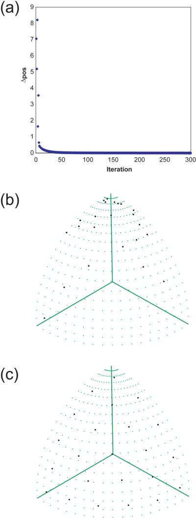
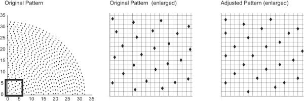
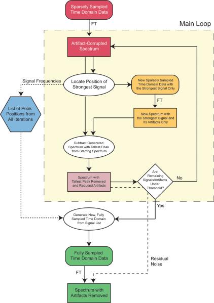
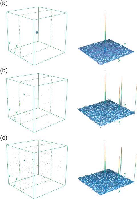
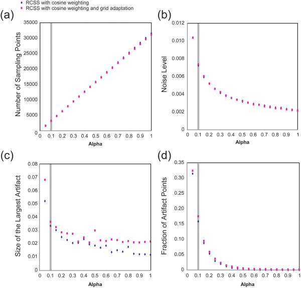
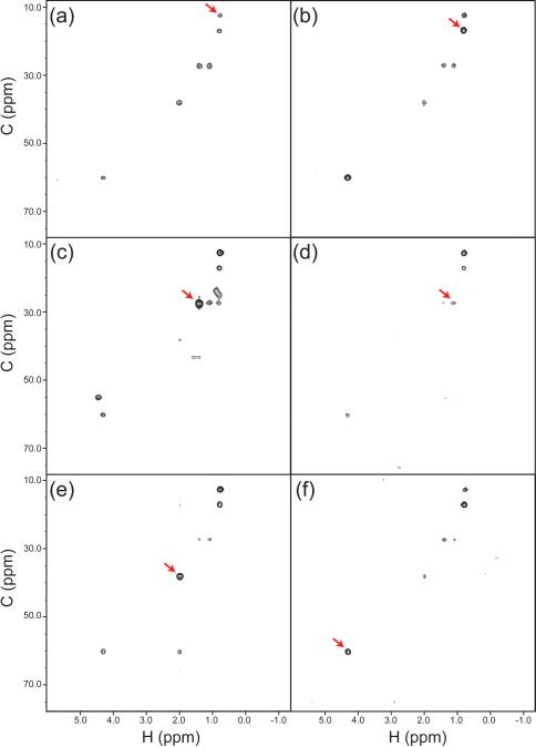
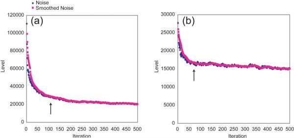
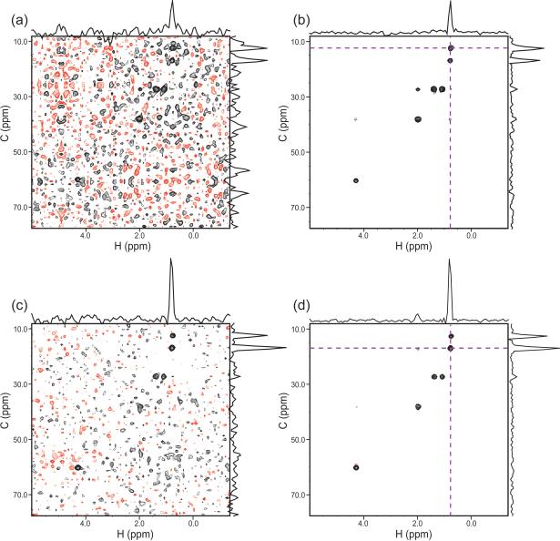
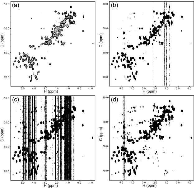
Recent efforts to reduce the measurement time for multidimensional NMR experiments have fostered the development of a variety of new procedures for sampling and data processing. We recently described concentric ring sampling for 3-D NMR experiments, which is superior to radial sampling as input for processing by a multidimensional discrete Fourier transform. Here, we report the extension of this approach to 4-D spectroscopy as Randomized Concentric Shell Sampling (RCSS), where sampling points for the indirect dimensions are positioned on concentric shells, and where random rotations in the angular space are used to avoid coherent artifacts. With simulations, we show that RCSS produces a very low level of artifacts, even with a very limited number of sampling points. The RCSS sampling patterns can be adapted to fine rectangular grids to permit use of the Fast Fourier Transform in data processing, without an apparent increase in the artifact level. These artifacts can be further reduced to the noise level using the iterative CLEAN algorithm developed in radioastronomy. We demonstrate these methods on the high resolution 4-D HCCH-TOCSY spectrum of protein G's B1 domain, using only 1.2% of the sampling that would be needed conventionally for this resolution. The use of a multidimensional FFT instead of the slow DFT for initial data processing and for subsequent CLEAN significantly reduces the calculation time, yielding an artifact level that is on par with the level of the true spectral noise.

Figure 1. Uniform Positioning of Points on a Sphere

An example with 23 points is shown. (a) Δ_pos, the sum over all points of the distance each point was moved during an iteration, plotted as a function of the iteration number. (b) Initial random configuration of the sampling points. (c) Final configuration. The distribution of the points is roughly uniform, with roughly even spacing between them. However, there is no “perfect” configuration for 23 points, and the pattern therefore shows asymmetries and subtle variations from exact uniformity.

Figure 2. Adaptation of Sampling Patterns to a Fine Grid

Schematic diagram showing the adjustment of points on a concentric ring sampling pattern to a fine grid. The grid spacing is approximately two times the spacing of the concentric rings.

Figure 3

Flow Chart for CLEAN

Figure 4. Point Responses for RCSS Patterns

In each case, a 3-D contour plot is provided at left, with the lowest contour at 3% of the peak height, and additional contours at 4%, 5%, 10%, 25% and 75%. The 2-D stacked plot at right shows a cross section through the X/Y plane. Each axis has a length that is twice the intended spectral width. (a) Pattern with α = 1.0 and 32 shells, for 10,415 points. The 3-D contour plot shows no artifacts at or above 3% of the peak height. The stacked plot shows a clear zone with no artifacts extending almost the full radius of the spectrum, with artifacts appearing as random noise outside of this circle. (b) Pattern with α = 0.1, 64 shells, cosine envelope weighting and adaptation to a 64 × 64 × 64 point grid, for 3,190 sampling points. There are some artifacts at the 3% level, but almost all are lower. The stacked plot shows that these low level artifacts look like noise and cover the entirety of the spectrum, with no visible clear zone. Aliasing (folding) artifacts from the grid adaptation are visible on some edges and faces of the spectrum. (c) Pattern with α = 0.075, 64 shells, cosine envelope weighting and adaptation to a 64 × 64 × 64 point grid, for 2,399 sampling points. The results are similar to (b), but with slightly larger artifacts.

Figure 5. Properties of RCSS Sampling Patterns

The data are measured from simulations of point responses conducted for α from 0.05 to 1.0 at 0.05 intervals. The grey bar marks the sampling used in the HCCH-TOCSY experiment. Artifacts are detected by subtracting from each point response a reference spectrum containing only the peak. (a) Number of sampling points. This quantity increases linearly with α for a given number of rings. (b) Apparent noise level, measured relative to the peak height. The noise level is calculated as described in the text. Because these data are measured from simulations, the noise level is in fact the artifact level, as there is no white noise contributing to the result. (c) Size of the largest artifact, measured relative to the peak height. Grid folding artifacts on the very edge of the spectrum are not included. (d) Fraction of artifact points. The number of points with artifacts greater than 1% is tabulated and divided by the total number of points in the spectrum.

Figure 6. Experimental Results for RCSS on an HCCH-TOCSY Spectrum

As an example, six different views of the Ile6 spin system are shown. In each case, the F1/F2 (h/c) correlations are shown at the F3/F4 (C/H) position in the 4-D spectrum corresponding to one of the crosspeaks (indicated by arrows). (a) The h/c plane at the H/C position H = 0.73 ppm, C = 12.6 ppm of Ile6 H^δ1/C^δ1. (b) H=0.78 ppm, C = 16.9 ppm for Ile6 H^γ2/C^γ2. (c) H = 1.35 ppm, C = 27.1 ppm for Ile6 H^γ12/C^γ1. (d) H = 1.05 ppm, C = 27.1 ppm for Ile6 H^γ13/C^γ1. (e) H = 1.96 ppm, C = 37.9 ppm for Ile6 H^β/C^β. (f) H = 4.27 ppm, C = 60.1 ppm for H^α/C^α.

Figure 7. CLEAN Progress

The graphs show the estimated noise level over the course of a CLEAN run for two 3-D cubes from the HCCH-TOCSY. The smoothed noise is computed with a 15-iteration window. The arrow indicates the point at which a 5% noise stabilization cutoff would be activated to stop the calculation. (a) H = 0.73 ppm, for Ile6 H^δ1. The stopping point is 111 iterations. (b) H = 0.78 ppm, for Ile6 H^γ2. The stopping point is 63 iterations.

Figure 8. Comparison of Results with and without CLEAN

(a) The plane from the 4-D HCCH-TOCSY at H = 0.73 ppm, C = 12.6 ppm (Ile6 H^δ1/C^δ1), for processing with the FT alone. (b) The same plane as in (a) after processing with CLEAN, plotted at the same contour level. The calculation was stopped automatically under the 5% noise stabilization criteria. (c) The plane at H=0.78 ppm, C = 16.9 ppm (Ile6 H^γ2/C^γ2), without CLEAN and (d) with CLEAN.

Figure 9. Results for the Full HCCH-TOCSY Spectrum

(a) The H/C HSQC spectrum of GB1. (b) A projection of the 4-D RCSS HCCH-TOCSY onto the H/C plane. The vertical stripes are the result of cubes that have an especially high level of artifacts. (c) The same as (b), but plotted at a contour level that is 55% lower. (d) The same as (c), at the same contour level, but after CLEAN.

References

1. Barna JCJ, Laue ED. Conventional and exponential sampling for 2D NMR experiments with application to a 2D NMR spectrum of a protein. J Magn Reson. 1987;75:384–389.
1. Barna JCJ, Laue ED, Mayger MR, Skilling J, Worrall SJP. Exponential sampling, an alternative method for sampling in two-dimensional NMR experiments. J Magn Reson. 1987;73:69–77.
1. Barna JCJ, Tan SM, Laue ED. Use of CLEAN in conjunction with selective data sampling for 2D NMR experiments. J Magn Reson. 1988;78:327–332.
1. Bretthorst GL. Nonuniform sampling: bandwidth and aliasing. In: Rychert JT, Erickson GJ, Smith CR, editors. Bayesian inference and maximum entropy methods in science and engineering. American Institute of Physics; 2001. pp. 1–28.
1. Coggins BE, Venters RA, Zhou P. Generalized reconstruction of n-D NMR spectra from multiple projections: application to the 5-D HACACONH spectrum of protein G B1 domain. J Am Chem Soc. 2004;126:1000–1001. - PubMed
Publication types