Profound context-dependent plasticity of mitral cell responses in olfactory bulb

Abstract

On the basis of its primary circuit it has been postulated that the olfactory bulb (OB) is analogous to the retina in mammals. In retina, repeated exposure to the same visual stimulus results in a neural representation that remains relatively stable over time, even as the meaning of that stimulus to the animal changes. Stability of stimulus representation at early stages of processing allows for unbiased interpretation of incoming stimuli by higher order cortical centers. The alternative is that early stimulus representation is shaped by previously derived meaning, which could allow more efficient sampling of odor space providing a simplified yet biased interpretation of incoming stimuli. This study helps place the olfactory system on this continuum of subjective versus objective early sensory representation. Here we show that odor responses of the output cells of the OB, mitral cells, change transiently during a go-no-go odor discrimination task. The response changes occur in a manner that increases the ability of the circuit to convey information necessary to discriminate among closely related odors. Remarkably, a switch between which of the two odors is rewarded causes mitral cells to switch the polarity of their divergent responses. Taken together these results redefine the function of the OB as a transiently modifiable (active) filter, shaping early odor representations in behaviorally meaningful ways.

Figure 1. Raw Data, Electrode Location, and Spike Sorting

(A) One second of raw data collected from a single electrode and filtered at 300–3,000 Hz. (B) Ventral view of a 3D reconstruction of the OB with benzaldehyde activation pattern [73] illustrating the approximate location and layout of the tips of the electrode array (black dots). (C) Wavelet coefficient that was (Helps) used (left) and not used (No Help) (right) for sorting of spikes thresholded from the channel shown in (A). Waveform descriptors, like wavelet coefficients, that create non-normal distributions of spikes are effective for grouping spikes into clusters. (D) Sorted waveforms displayed with corresponding ISI histograms. The red unit was classified as a single unit because it displayed less than 3% of total spikes violating an ISI less than 2 ms (see Materials and Methods). (E) Histogram showing the distribution of prestimulus firing frequencies for 660 units (189 single units and 471 multi units). The red histogram is the distribution for the single units (18.5 ± 5 Hz, n = 189, mean ± SD), and the blue histogram is the distribution for the multi units (94 ± 33 Hz, n = 471).

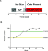
Figure 2. Go–No-Go Odor Discrimination Task.

(A) Time course for each trial in the odor discrimination task. The trial is started by a nose poke of the mouse into the odor chamber. When the computer senses the nose poke it turns a valve that diverts the air flow of 2 l/min to the exhaust and it turns on the odor valve that injects odorized air into the main air flow at 40 ml/min. The mouse must remain in the chamber for a time period made up of a variable 0–0.5-s period (variable diverting valve period or vDV) followed by a fixed 1-s interval (fDV). At the end of the fixed diverting valve (fDV) period the odor has mixed thoroughly with the main air flow, and the diverting valve directs the air flow back into the chamber (time 0 s). At this time the mouse must stay for 0.5 s in the chamber (S) and then must lick at least once in each of the 0.5-s response area (RA) segments if the odor is a rewarded odor. If the mouse licks in the four RA segments, the mouse is rewarded with water flowing through the tube it has been licking. A 6-s time out follows the end of the trial. If the odor is an unrewarded odor the mouse does not have to lick, and typically withdraws the head from the odor port shortly after it makes a decision. While the diverting valve is activated at time zero, there is a delay in delivery of the odor that we estimate to be of the order of ∼300 ms. (B) Typical curve for behavioral performance in an odor discrimination session. The percent correct response is shown as a function of block number. Each block includes ten rewarded odor and ten unrewarded odor trials. A correct response is licking of the tube in the four RA segments for a rewarded odor and not licking in at least one RA period for the unrewarded odor (this is the go–no-go criterion). Note that this mouse starts with chance performance (50%) and reaches the arbitrary response criterion of 85% correct by four blocks.

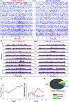
Figure 3. Divergence in Single Unit Responses during Learning in the Odor Discrimination Task

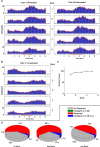
(A) Raster plot of single unit spike times organized per block for the ten rewarded trials (A, left column) and ten unrewarded trials (AB, right column). Timing and duration of odor exposure is indicated on the x-axis by the red bar. (B) PSTH of the data shown in (A). Red lines on either side of the histogram indicate +/− standard error of the mean (SEM). The bin size in the PSTH is 0.15 s. This means that the firing rate in Hz is the value in the y-axis × (1/0.15). (C) Behavioral performance—percent correct as a function of block number—for the animal from whom the cell in (A) and (B) was recorded. (D) A plot of the firing-rate increase above background to odor A (red) and odor AB (blue) in each block of the behavior. The points represent the firing rate in spikes/0.15-s bin during odor exposure (0.5 to 2.5 s) minus the rate in spikes/0.15-s bin in the period immediately before odor exposure (−1 to 0 s). Error bars denote the mean +/− SEM of each point (ten trials per point). (E) The lower right hand pie chart shows what percent of the responses were inhibitory (gray), excitatory (yellow), or mixed (blue). A mixed response was defined as a response to either odor A or AB that had both an excitatory and inhibitory component or a response that was excitatory to one odor and inhibitory to the other odor stimulus.

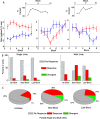
Figure 4. Transient Firing Changes Observed during Learning

(A) The top black plots display the behavior of the animal from which the unit data displayed in the lower plots was recorded. The behavior plot on the left corresponds to the two plots in the lower left and the upper right behavioral plot goes with the lower right rate change plot. The lower plots show unit firing rate change in response to odor A (red/rewarded) and odor AB (blue/ unrewarded) in each block of the behavior. The points represent the firing rate in spikes/0.15-s bins during odor exposure (0.5 to 2.5 s) minus the rate in spikes/0.15-s bin in the period before odor exposure (−1 to 0 s) (for details see Materials and Methods). Error bars denote mean +/− SEM of each point. (B) Bar graphs depicting the percent of total units that were responsive(red) and divergent (green) in the first, best, and last blocks. The data are from 189 single units (left) and 471 multiunits (right) recorded from eight different animals in 38 sessions. (C) The three pie charts illustrate the percent of total units (pooled single and multiunits) that were responsive (red) and divergent (green) in the first, best, and last blocks. The data are from 660 units recorded from eight different animals and 38 separate odor discriminations.

Figure 5. Lick and Odor Responses Where the Animal Made Correct or Incorrect Behavioral Responses

(A) Trial by trial rasters of lick behavior for the rewarded (odor A, left) and unrewarded (odor AB, right) odors. Red indicates periods of licking and blue indicates periods of no licking. Data for ten trials are shown for rewarded and unrewarded odors per block. Blocks are arranged from top to bottom. The green bar below the rasters indicates when the odor was delivered to the chamber. The yellow arrows point to trials where the animal made a mistake in the lick response. (B) Histograms of response magnitude normalized to the average correct rewarded (1) and unrewarded (0) firing rates during the peristimulus period sorted for the four different types of behavioral outcomes. The normalized response magnitude was calculated for each unit for all divergent units in 11 sessions in four animals (these were a subset of the 34 sessions in Figure 4 where the animal made six or more mistakes). Hits are trials where the animal licks sufficiently to obtain a water reward during a rewarded odor trial. Misses are trials in which the animal fails to lick sufficiently to receive reward on rewarded odor trials. Correct rejections (CR) are trials in which the animal refrains from licking during an unrewarded odor trial. False alarms (FA) are trials in which the animal responds by licking to an unrewarded odor as if it were a rewarded trial. The number of counts per bin represents the number of units displaying a response of a given normalized magnitude.

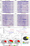
Figure 6. Changes in MC Odor Responses during Reversal

(A) PSTH for a multiunit response to odors A and AB during an initial discrimination (day 1) whose behavioral performance curve (percent correct responses versus block number) is displayed in (D) (left). This unit never develops a significant response to A but develops a significant inhibitory response to AB. (B) The same multiunit responding the next day (day 2) in the performance of a reversal task in which the reward associations of odor A and AB had been reversed (the behavioral curve is displayed in the right side of [D]). The unit developed a significant inhibitory response to odor A (now unrewarded) and a significant excitatory response to odor AB (now rewarded). The red bar under the time axis denotes the interval when the mouse was exposed to the odor. (C) Odor-elicited firing-rate changes observed during day 1 (left) and during reversal in day 2 (right). The two plots show unit firing-rate change in response to odor A (red) and odor AB (blue) in each block of the session. The points represent the firing rate in spikes/0.15-s bins during odor exposure (0.5 to 2.5 s) minus the rate in spikes/0.15-s bin in the period before odor exposure (−1 to 0 s) (for details see Materials and Methods). Error bars denote mean +/− SEM of each point (n = 10 rewarded and 10 unrewarded odors per block). An ANOVA indicated that in both day 1 and day 2 the responses to odor A differed from responses to odor AB (p < 0.05). (D) Percent correct responses for the behavior in the first day task (left) and the second day reversal (right). (E) Summary of all reversal experiments consisting of 358 units from eight animals and 24 different reversal sessions. (F) Pie illustrating what happens to units that are divergent in either the initial discrimination or the reversal. “No Divergent Pair” indicates that the unit only had statistically significant divergence in one of the two complementary tasks. “Valence Switch” means that the odor evoked firing rates switched from A>AB to AAB to A>AB or vice versa from the initial discrimination to the reversal.

Figure 7. Responses of SMCs to Novel Rewarded Odors A and AB in the Multiple S+ Control Task Do Not Diverge between A and AB

(A) PSTH of a multiunit response to odor A (left) and AB (right) both of which are rewarded. This multiunit responds to both odors A and AB with a significant excitatory response. (B) PSTH of the same unit responding to the unrewarded odor C (cumin aldehyde) that the animals were familiar with as an unreinforced stimulus prior to start of the task. This unit displays a significant inhibitory response to odor C. There are twice as many trials of odor C compared to A and AB per block because the ratio of rewarded to unrewarded odors remains at 50% in this task. For every ten trials of odor A or Odor AB there are 20 trials of odor C. (C) Behavior plot corresponding to the raster shown in (A) and (B). It should be noted that the animal performs at criterion from the first block because although odors A and AB are novel, odor C has an overtrained association as the unrewarded stimulus. (D) Summary of all experiments consisting of 200 units from six animals and 12 different task sessions. It should be recognized that the green pie denoting units divergent in A versus AB responses do not exist in this behavior. The added blue pie piece signifies the percent of total units that had a divergent response between either A or AB and odor C. This value did not significantly vary through the course of the task (first, best, and last).

Figure 8. Behavioral Decision and Unit Divergence Times

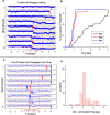
(A) This figure shows the p-value of the difference between the lick responses in rewarded and unrewarded trials calculated for each block for the data shown in Figure 5A using a rank sum test at each 0.15-s bin through the trial. As shown in Figure 5A each bin is allocated a value of 1 if the mouse licked at least once or a value of zero if the mouse did not lick. The rank sum test is performed on all zeros and ones in each bin within each block. The vertical red lines indicate when the p-value drops below 0.05. The horizontal red lines indicate the 0.05 level. The blocks are shown from top (first block) to bottom (last block). (B) Percent cumulative probability plot summarizing the decision times for the 19 go–no-go experiments where at least one unit diverged when the response to the reinforced and unreinforced odors were compared (the experiments contributing to the green wedge in the pie charts in Figure 4B). The decision time becomes smaller as the animal progresses through the session as evidenced by a shift of the median decision time from 2.5 s for the first block, to 1.0 s for the best block, and 0.95 s for the last block. It is important to state that as explained in the Materials and Methods the actual time of arrival of the odor is delayed ∼300 ms, and therefore what is important in this experiment is not the absolute value of the decision times but rather the relative values. (C) Plot of the p-value of the difference between firing rates between odor A trials and odor AB trials compared at different times throughout the trial for the unit shown in Figure 3A. p-Values were calculated by using a rank sum test applied to the firing rate calculated in each block in each 0.15-s bin. The horizontal red line is drawn at a p-value of 0.05. The vertical blue lines indicate the time at which the difference in firing rate between odor A and AB dropped below 0.05 for two or more consecutive points. Because of multiple comparisons, the p-value falls below 0.05 occasionally for a single point as seen by the few single data points that fall below the red line in the period before odor responses (−2 to 0 s). We found that two adjacent data points fall below 0.05 only rarely in this prestimulus period (4% of the time) allowing us to use the criterion of two adjacent points below 0.05 as the time when the two rates differ. The vertical red lines are taken form (B) and allow for a comparison of timing between divergent lick behavior and divergent MC firing. (D) Distribution of the difference between unit divergence times and their corresponding behavioral decision times during the best block. The majority of unit divergence occurs after the animal has begun divergent licking behavior (positive values). Only 20% of the units diverge in their firing rate responses to the rewarded and unrewarded odor prior to behavioral divergence of licking.

Figure 9. PCA of the Responses of the 95 Divergent SMCs Calculated for the First, Best, and Last Blocks

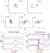
The input to the PCA was the number of spikes per 0.15-s bin for all the trials in each block for the 95 divergent SMCs. The PCA algorithm computes principal components (linear combinations of the input variables) ranked in order of how much of the variance they account for in the dataset; the first few principal components (PC1 and PC2 are shown in [A] and [B]) explain most of the variance and they can be thought of as the firing rate of newly formed units containing a large amount of the information on odor divergence. Note that the principal components are dimensionless and therefore, no units are shown in the graphs. (A) Scatterplots displaying points denoting the location in two-dimensional principal component space of each trial in the best block. The left panel displays the distribution of points at a time before exposure to odor (−0.3 s) and the right panel shows the distribution at a time point during odor exposure (1.5 s). The red points are trials where the animals were exposed to the reinforced odor and the blue points are trials with the unreinforced odor. (B) The entire mean trajectory through time in two -dimensional principal component space is shown for the first (left), best (center), and last (right) blocks. In order to generate the mean trajectory, the mean location of all red and blue points in graphs such as those shown in (A), but spanning the entire time course from −2.5 to 4.5 s was calculated and plotted as a continuous line. Zero seconds is the time when the diverting valve is turned off and the odor is directed towards the animal. The red line is the trajectory for trials with the reinforced odor and the blue line is the trajectory for trials with the unreinforced odor. The trajectories hover around the origin (0.0) during the period before the odor valve opens (It < 0 s) and then move outward in opposite directions after the diverting valve is opened (0 to 2.5 s) during the period when the animal is exposed to the odor. The numbers adjacent to specific points in the trajectory for the best block denote different times in the trial and are shown to facilitate understanding of how the points move through time. The numbers stand for the following times: (1) 0.75 s; (2) 1.05 s; (3) 1.65 s; (4) 2.1 s. (C) The blue line shows the change during the time course of a trial of the mean of all pairwise euclidean distances in PCA space between points that belonged to trials where the animals were exposed to different odors (reinforced versus unreinforced odors). Pairwise euclidean distances are calculated in 95-dimensional principal component space. To calculate the delta distances shown by the blue line the mean of the pairwise distances between points for trials where the animals were stimulated with the same odor were subtracted from the mean of pairwise distances for points for trials where animals were stimulated with different odors. The red traces represent the SEM. (D) Logarithm of the p-value calculated with a rank sum test performed at every 0.15-s time bin for the difference in the pairwise PCA distances between points for trials where the animals were stimulated with the same odor compared to pairwise distances for points for trials where animals were stimulated with different odors. If the logarithm of the p-value fell below −5, the point was assigned a value of −5. The horizontal red line is the logarithm of 0.05. The vertical black lines are the times when the p-value drops below 0.05, and the red vertical lines are the median of the behavioral discrimination times shown in Figure 8B.

References

1. Mombaerts P, Wang F, Dulac C, Chao SK, Nemes A, et al. Visualizing an olfactory sensory map. Cell. 1996;87:675–686. - PubMed
1. Buck L, Axel R. A novel multigene family may encode odorant receptors: a molecular basis for odor recognition. Cell. 1991;65:175–187. - PubMed
1. Malnic B, Hirono J, Sato T, Buck LB. Combinatorial receptor codes for odors. Cell. 1999;96:713–723. - PubMed
1. Shepherd GM, Chen WR, Greer CA. Olfactory bulb. In: Shepherd GM, editor. The synaptic organization of the brain. New York: Oxford University Press; 2004. pp. 159–204.
1. Mori K, Takahashi YK, Igarashi KM, Yamaguchi M. Maps of odorant molecular features in the Mammalian olfactory bulb. Physiol Rev. 2006;86:409–433. - PubMed
Publication types