. 2008 Oct;62(10):2451-61.
doi: 10.1111/j.1558-5646.2008.00472.x.

Understanding the evolution and stability of the G-matrix

Affiliations

Understanding the evolution and stability of the G-matrix

Stevan J Arnold et al. Evolution. 2008 Oct.

Abstract

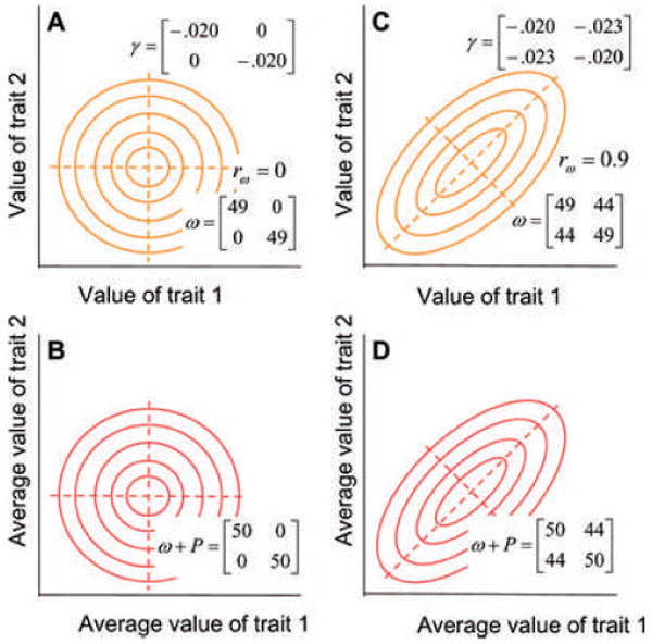
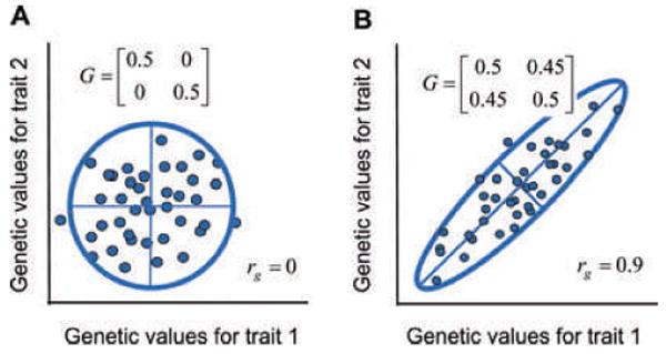
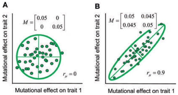
The G-matrix summarizes the inheritance of multiple, phenotypic traits. The stability and evolution of this matrix are important issues because they affect our ability to predict how the phenotypic traits evolve by selection and drift. Despite the centrality of these issues, comparative, experimental, and analytical approaches to understanding the stability and evolution of the G-matrix have met with limited success. Nevertheless, empirical studies often find that certain structural features of the matrix are remarkably constant, suggesting that persistent selection regimes or other factors promote stability. On the theoretical side, no one has been able to derive equations that would relate stability of the G-matrix to selection regimes, population size, migration, or to the details of genetic architecture. Recent simulation studies of evolving G-matrices offer solutions to some of these problems, as well as a deeper, synthetic understanding of both the G-matrix and adaptive radiations.


Figures

Figure 1
Figure 1
Individual selection surfaces and adaptive landscapes for two phenotypic traits can be represented by matrices or contour plots. The plots illustrate two kinds of bivariate stabilizing selection. Eigenvectors (principal components) are shown with dashed lines. The bivariate phenotypic mean is situated at the adaptive peak (intersection of the dashed lines) and consequently there is no directional selection. (A) An individual selection surface with weak stabilizing selection on each trait (γ11 = γ22 = −0.20) but no correlational selection (γ12 = 0). In this plot, expected individual fitness (contours) is a function of trait values. Because the curvature of this surface is weak, it can be approximated by a bivariate Gaussian surface described by the ω-matrix. (B) The adaptive landscape corresponding to the individual selection surface described in (A). In this plot, average population fitness (contours) is a function of average trait values. P is the within-population variance–covariance matrix before selection. The elements in the illustrated case are P11 = P22 = 1, P12 = P21 = 0. (C) An individual selection surface with weak stabilizing selection on each trait and positive correlational selection (ω12 = 44, rω = 0.9). (D) The adaptive landscape corresponding to (C). The P-matrix is the same as in (B). Note that in these examples, the AL and the ISS have similar curvature and orientation because selection is weak (i.e., ω-matrix is large) relative to the P-matrix.
Figure 2
Figure 2
The distribution of additive genetic values for two traits can be represented as a cloud of values or a matrix, G. Same conventions as in Figure 2. (A) A data cloud with no genetic correlation (rg = 0). (B) A data cloud with a strong positive genetic correlation (rg = 0.9).
Figure 3
Figure 3
The distribution of new mutational effects on two traits from a particular locus can be represented as a cloud of values or a matrix, M. The 95% confidence ellipses for each data cloud are shown. The axes inside each ellipse are eigenvectors (principal components). (A) A cloud of mutations with no correlation (rμ = 0). (B) A cloud of mutations with a strong positive correlation in mutational effects (rμ = 0.9).
Figure 4
Figure 4
The Flury hierarchy for comparing G-matrices is a nested series of hypotheses that are tested by comparing eigenvectors and eigenvalues. The hypotheses are listed on the left and depicted on the right with 95% confidence ellipses. From top to bottom, the hypotheses are: (A) equal matrices (eigenvectors equal, eigenvalues equal), (B) proportional matrices (eigenvectors equal; eigenvalues proportional), (C) matrices with common principal components, CPC (eigenvectors equal, eigenvalues not equal), and (D) unrelated matrices (eigenvectors and eigenvalues not equal). For more than n = 2 traits, an additional possible hypothesis is partial CPC, in which up to n − 2 eigenvectors are shared among matrices, but the remaining eigenvectors differ.
Figure 5
Figure 5
Graphical summary of the results of empirical comparisons of G-matrices. Only 31 studies that made comparisons with the Flury hierarchy are included here. From left to right, the four panels refer to studies that compared experimental populations of the same species that have been exposed to different environmental treatments (n = 63 pairwise comparisons), males and females from the same population (n = 12), conspecific populations sampled from nature (n = 97), or different species sampled from nature (p = 32). The outcomes of statistical tests are classified into categories described in Figure 4. Full CPC means that matrices had all principal components (eigenvectors) in common) partial CPC means at least one but not all principal components are in common. Some studies compared multiple pairs of matrices. In such cases, all of the outcomes are tabulated.
Figure 6
Figure 6
Evolution and stability of the G-matrix in response to different patterns of mutation and selection (stationary optimum). Each row shows the results (snapshots) from a single simulation run lasting 2000 generations. The first three ellipses in each row are the 95% confidence ellipses (or equivalent) for the M-matrix, the adaptive landscape (ω + P matrix), and the resulting average G-matrix (n = 2000 generations). These three ellipses are shown on different scales. The average G-matrix is the reference size, but the M-matrix is magnified by a factor of 3, and the ω + P matrix is reduced by a factor of 10. The average P-matrix (n = 2000 generations) was added to the ω-matrix to compute the ω + P matrix. The last eight ellipses in each row show snapshots of the G-matrix (95% confidence ellipses) every 200 generations, shown at the same scale as the average G-matrix. From top to bottom, the values of mutation and selection and the resulting average genetic correlation are: (A) rμ = rω = 0, rg = −0.09. (B) rμ = 0, rω = 0.75, rg = 0.29. (C) rμ = 0.50, rω = 0, rg = 0.48. (D) rμ = 0.50, rω = 0.75, rg = 0.64. (E) rμ = 0.90, rω = 0.90, rg = 0.93. The following parameters are the same for all rows: Ne = 342, ω11 = ω22 = 49, and the mutational variances for each character are 0.05 (as in Fig. 3).
Figure 7
Figure 7
Contrasting conditions can promote instability or stability of the G-matrix on an adaptive landscape with a moving optimum. Results from simulations using the Jones et al. (2004) program are shown in this figure. In both cases the peak of the adaptive landscape (solid red dot) has moved from the bottom left to the upper right at the same rate. Peak position is shown every 300 generations. The bivariate phenotypic mean (intersection of the axes of the G-matrix, shown as a blue ellipse) tracks the moving peak and is also shown every 300 generations. Effective population size is relatively small (Ne = 342). (A) No correlated pleiotropic mutational effects (shown as a circular green ellipse, rμ = 0) and no correlational selection (shown as a circular adaptive landscape, red contours, rω = 0) promote instability of the G-matrix. Notice that G (blue ellipses) changes in size, shape, and especially in orientation from snapshot to snapshot. (B) Strong mutational correlation (rμ = 0.9) and strong correlational selection (rω = 0.9), combined with peak movement along the selective line of least resistance, promote stability in the size, shape, and orientation of the G-matrix. Notice that the cigar-shaped G-matrices hardly vary from snapshot to snapshot. Although the three stability-promoting conditions are combined here, other simulations show that they make individual contributions to the stability and evolution of the G-matrix.
Figure 8
Figure 8
The M-matrix tends to evolve toward alignment with the adaptive landscape. This figure summarizes the results of simulations in which one feature of the M-matrix, the mutational correlation (rμ), was allowed to evolve as the orientation of the adaptive landscape was varied. In different runs the selectional correlation (rω) was held constant at 0.90 by systematically varying the elements of the ω-matrix, so that the orientation of the leading eigenvector of the adaptive landscape (angle of correlational selection) varied from about 19–45 degrees (replotting of data shown in Fig. 5 of Jones et al. 2007). Each point represents the mean of 50 replicate runs (± SE).

References

    1. Arnold SJ. Constraints on phenotypic evolution. Am Nat. 1992;140:S85–S107. - PubMed
    1. Arnold SJ, Phillips PC. Hierarchical comparison of genetic variance covariance matrices. II. Coastal-inland divergence in the garter snake, Thamnophis elegans. J Evol Biol. 1999;53:1516–1527. - PubMed
    1. Arnold SJ, Pfrender ME, Jones AG. Tire adaptive landscape as a conceptual bridge between micro- and macroevolution. Genetica. 2001:112–113. 9–32. - PubMed
    1. Baatz M, Wagner GP. Adaptive inertia caused by hidden pleiotropic effects. Theor Pop Biol. 1997;5:49–66.
    1. Barton N, Keightley PD. Understanding quantitative genetic variation. Nat Rev Genet. 2002;3:11–20. - PubMed

Publication types