Continuous shifts in the active set of spinal interneurons during changes in locomotor speed

Abstract

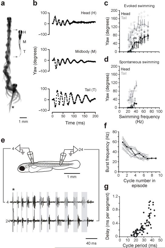
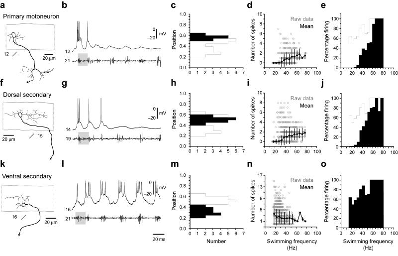
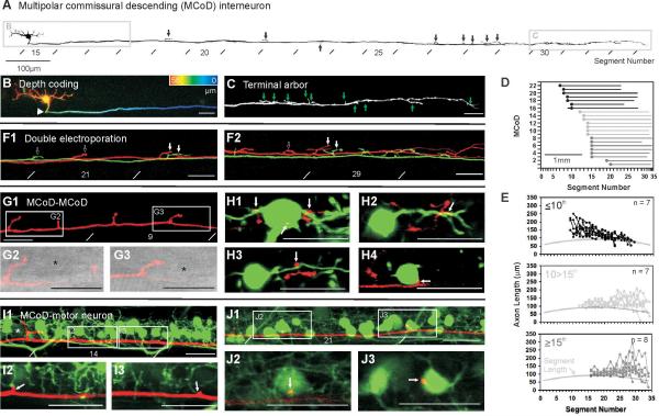
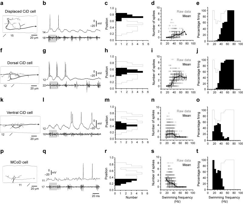
The classic 'size principle' of motor control describes how increasingly forceful movements arise by the recruitment of motoneurons of progressively larger size and force output into the active pool. We explored the activity of pools of spinal interneurons in larval zebrafish and found that increases in swimming speed were not associated with the simple addition of cells to the active pool. Instead, the recruitment of interneurons at faster speeds was accompanied by the silencing of those driving movements at slower speeds. This silencing occurred both between and within classes of rhythmically active premotor excitatory interneurons. Thus, unlike motoneurons, there is a continuous shift in the set of cells driving the behavior, even though changes in the speed of the movements and the frequency of the motor pattern appear to be smoothly graded. We conclude that fundamentally different principles may underlie the recruitment of motoneuron and interneuron pools.

Figure 1. Analysis of real and fictive evoked swimming movements

(a) Consecutive overlapping images of a bout of swimming elicited by a tactile stimulus to the tail (at asterisk). A frame extracted from the montage (gray arrows) shows the regions selected for kinematic analysis, at the head (H), midbody (M) and tail (T). Images were captured at 1,000 Hz (images 1-9, every 4 ms; 10-12, 8 ms; 13-14, 16 ms; 15-18, 32 ms). (b) Automated analysis of yaw at three points along the body, from the swimming bout illustrated in a. Only the tail is showing any noticeable movement at the end of the bout, when swimming is slowest. (c) Plots of head and tail yaw from 12 evoked swimming bouts in 12 larvae. The degree of head and tail yaw decreases as a function of swimming frequency. Open circles are raw data points, while closed circles represent means (plus or minus standard deviations) from data binned at 5 Hz intervals (e.g., 15-20, 20-25, etc...). For simplicity, only the first episode of the five analyzed in each fish is illustrated here and in d (see Methods). (d) A similar plot for spontaneous bouts of swimming (12 from the same 12 larvae), whose values are comparable to the lower end of evoked swimming frequencies. (e) Fictive swimming activity recorded from motor nerves along the same side of the body (4^th and 24^th muscle cleft on the left side), whose location is illustrated schematically. A brief electrical stimulus (artifact at asterisk) was used to elicit swimming activity. Shaded gray boxes from the start of the burst in the rostral segment to the start of the caudal burst in the same cycle demonstrate the gradual increase in longitudinal delay associated with a smooth decrease in swimming frequency. (f) Plot of motor nerve burst frequency (measured from the tail) with respect to the cycle in a bout, from 10 bouts in 10 larvae. (g) Plot of longitudinal delay with respect to cycle period, from the same 10 bouts in f.

Figure 2. Recruitment pattern of spinal motoneurons

(a-e) Data from primary motoneurons are organized according to morphology (a), physiology (b), dorso-ventral soma position (c), number of spikes during swimming at different frequencies (d) and reliability of firing during swimming at different frequencies (e). In a, a black arrow indicates continuation of the axon. Segment locations are noted below the images. In b, gray shaded boxes are present to illustrate a similar swimming frequency. Segmental recording locations are noted to the left of the trace. For reference, in c and e, a gray outline shows the maximum values of the histogram one would get if those for the individual groups of neurons were overlain. In d, open circles are raw data points, while closed circles represent means (plus and minus standard deviations) from data binned at 5 Hz intervals, using the nerve recording as a frequency reference. In e, the number of cycles in which a cell fired is expressed as a percentage of the total number of cycles at that frequency. Plots are derived from 173 bouts from 10 cells in 10 larvae. (f-j) Data from dorsally located secondary motoneurons (> 0.42) are organized as detailed in a-e. Plots are derived from 317 bouts from 16 cells in 16 larvae. (k-o) Data from more ventrally located secondary motoneurons (< 0.42) are organized as detailed in a-e. Plots are derived from 187 bouts from 14 cells in 14 larvae.

Figure 3. Anatomy of multipolar commissural descending (MCoD) interneurons

(a) Inverted fluorescent image of a dye-filled MCoD created from successive confocal images along the body. Black arrows indicate axon collaterals, lines indicate myomeric segmental boundaries. (b) The contralateral axonal projection characteristic of MCoDs is illustrated here by pseudocoloring the region in a according to depth (red is distal and blue is proximal, total depth is 58 μm). (c) Magnification of the region indicated in a provides a more detailed view of axon collaterals (at green arrows). This image is created from a collapsed Z-stack 18 μm in thickness. (d) Plot of the length of descending axons for 22 electroporated MCoDs. The X-axis has been normalized according to the length of each muscle segment. (e) Plots of axon lengths per segment (in micrometers) for MCoDs located in three defined segmental regions (as indicated on the respective plots). Here, the X-axis has not been normalized to segment lengths. For comparison, a gray line indicates the length of each segment. (f-g) MCoDs located in either the 9^th (red) and 11^th (green) segments (f) or the 14^th (red) and 15^th (green) segments (g) were electroporated with different wavelength dyes to examine the relationship of axon collaterals. White arrows indicate potential sites of convergence, while open arrows indicate likely sites of divergence. f is a collapsed Z-stack 9 μm thick, while g is 14 μm thick. (h-j) A confocal image of a MCoD electroporated in the 7^th segment (h), when combined with differential interference contrast (DIC) light microscopy (i and j), reveals the proximity of axon collaterals to somata located laterally in the neuropil (at asterisks), where they might contact processes arising from the somata. h is a collapsed Z-stack 12 μm thick, while i and j are single 1 μm optical sections. (k-n) Confocal images of an electroporated MCoD (red) from the 9^th segment and back-filled MCoDs (green) from the 13^th (k), 14^th (l), 15^th (m) and 16^th (n) segments reveal the proximity of MCoD axon collaterals (at white arrows) to the dendrites and somata of more caudal MCoDs on the opposite side of the body. Images are single 1 μm optical sections. (o-q) Confocal images of Islet-1 GFP (green) labeled secondary motoneurons and an electroporated MCoD (red) from the 12^th segment. The MCoD axon runs along the ventral extent of the dendritic zone (o), where it appears to make contact with dendrites (p and q). o is a collapsed Z-stack 13 μm thick, while p and q are single 1 μm optical sections. (r-t) Confocal images as described in o-q, but nearer the tail. The MCoD here is from the 13^th segment. More caudally, the MCoD axon runs at the level of secondary motoneuron somata (r), where axon collaterals appear to make direct somatic contact (s and t). r is a collapsed Z-stack 15 μm thick, while s and t are single 1 μm optical sections. All scale bars are 20 μm, unless labeled.

Figure 4. Pair-wise recordings of MCoDs and motoneurons

(a) Graphic reconstructions of the connected MCoD and secondary motoneuron (smn; see top schematic for respective location), whose physiology is illustrated in b. The MCoD axon crosses the spinal cord (at asterisk) and descends contralaterally (gray). The secondary motoneuron axon was torn during the dissection (asterisk). Segment locations are indicated below the images. (b) Five overlapping traces of post-synaptic potentials (PSPs) in a secondary motoneuron (smn) from the 29^th segment following spikes generated in a MCoD from the 13^th segment in control conditions (top gray trace), in high divalent cation solution (middle gray trace) and following the blockade of glutamatergic synapses with 10 μM NBQX and 100 μM APV (bottom gray trace). A black arrow highlights the likely electrical component of the PSP. For simplicity, only one action potential trace is shown (top black trace).

Figure 5. Rhythmic firing behavior of MCoDs during fictive swimming

(a-b) Spontaneous bouts of fictive swimming while recording from a MCoD and a motor nerve are illustrated on a slower (a) and faster (b) time base. Segmental locations are noted on the traces. (c) Recordings of bouts of swimming from a different larva illustrate that at higher swimming frequencies MCoDs are less likely to fire action potentials. (d) Plot of the number of spikes in a MCoD per cycle versus swimming frequency using the nerve recording as a frequency reference (287 swimming bouts in 10 larvae). Open circles are raw data points, while closed circles represent means (plus standard deviations) from data binned at 5 Hz intervals. (e) Histogram of swimming frequency measured from nerve recordings of 1,896 cycles from 287 swimming bouts in 10 larvae.

Figure 6. Inhibition of MCoDs at fast swimming frequencies

(a-b) Recordings of a MCoD and a motor nerve in response to a brief electrical stimulus (at asterisk) at two depolarized holding potentials, one using 10 pA of current (a) and one using 20 pA (b). Holding the MCoD at a more depolarized level reveals the hyperpolarizing nature of the inhibition early in the bout when the frequency of swimming is highest (at gray arrows). (c-d) Recordings in cell-attached mode (c) and whole-cell mode (d). The MCoD is inhibited at the beginning of the episode when swimming is fastest using both approaches. Spikes in cell-attached mode are marked by black arrows. These recordings were routinely performed to make sure the inhibition was not simply an artifact of our patch recording process. (e-h) The inhibition of the MCoD at faster swimming frequencies (e) can be reversibly blocked by strychnine (f), suggesting it is glycinergic. With prolonged exposure (g), strychnine also disrupts the motor pattern as assessed by the motor nerve recording. This effect is reversed when returned to control saline (h).

Figure 7. Dual MCoD and CiD interneuron recordings

(a) Graphic reconstructions of the MCoD (gray) and CiD (black) whose physiology is illustrated in b. A black asterisk indicates where the MCoD axon crosses cord, while arrows indicate the continuation of the axons. (b) Whole-cell recordings from a MCoD and CiD in the same segment with mutually exclusive firing behavior. Simultaneous cyclical firing behavior was extremely rare (5 out of 223 cycles from 43 swimming bouts in 4 larvae). For frequency measures, cells must fire in consecutive motor bursts to be quantified. Using this criterion, events were only counted as simultaneous if the MCoD and CiD both fired cyclically, in the same two consecutive bursts of motor output. Here, gray lines mark the transition at which the CiD stopped firing and the MCoD began. In this case, the MCoD and CiD only fired together during one burst at the transition and so by our definition are not synchronous. (c) Plot of firing of MCoD/CiD pairs in different trials versus swimming frequency, using the inter-cycle interval of the MCoD (open gray circles) or the CiD (filled black circles) firing as the frequency measure, from 43 swimming bouts in 4 larvae in which MCoD and CiD pairs were recorded. Black boxes illustrate examples where the MCoD and the CiD fired in the same cycle, which was very rare.

Figure 8. Frequency-dependent shifts in recruitment within and between classes

(a-e) Data from displaced, dorsally located CiD cells, the most dorsal of the CiDs, are organized according to morphology (a), physiology (b), dorso-ventral soma position (c), number of spikes during swimming at different frequencies (d) and reliability of firing during swimming at different frequencies (e). In a, black arrows indicate continuation of the axon. Segment locations are noted below the images. In b, gray shaded boxes are present to illustrate a similar swimming frequency. Segmental recording locations are noted to the left of the trace. For reference, in c and e, a gray outline shows the maximum values of the histogram one would get if those for the individual groups of neurons were overlain. In d, open circles are raw data points, while closed circles represent means (plus and minus standard deviations) from data binned at 5 Hz intervals, using the nerve recording as a frequency reference. In e, the number of cycles in which a cell fired is expressed as a percentage of the total number of cycles at that frequency. Plots are derived from 127 bouts from 12 cells in 12 larvae. (f-j) Data from dorsally located, non-displaced CiD cells are organized as detailed in a-e Plots are derived from 268 bouts from 14 cells in 14 larvae. (k-o) Data from more ventrally located CiD cells are organized as detailed in a-e. Plots are derived from 398 bouts from 11 cells in 11 larvae. (p-t) Data from MCoD cells are organized as detailed in a-e In p, an asterisk marks where the axon crosses cord and then descends. The plot in s was first illustrated in Figure 5d. As the frequency of swimming increases, the active set of cells shifts from the ventral MCoDs and CiDs to the dorsal CiDs, as seen most easily by a comparison of the positions (black bars superimposed upon the whole population outlined in gray in c, h, m, r) with the frequencies over which they are active (black in e, j, o, t).

Figure 9

References

1. Mendell LM. The size principle: a rule describing the recruitment of motoneurons. J Neurophysiol. 2005;93:3024–3026. - PubMed
1. Cope TC, Sokoloff AJ. Orderly recruitment among motoneurons supplying different muscles. J Physiol Paris. 1999;93:81–85. - PubMed
1. Cope TC, Pinter MJ. The size principle: Still working after all these years. News in Physiological Sciences. 1995;10:280–286.
1. Henneman E, Somjen G, Carpenter DO. Functional Significance of Cell Size in Spinal Motoneurons. J Neurophysiol. 1965;28:560–580. - PubMed
1. Zajac FE, Faden JS. Relationship among recruitment order, axonal conduction velocity, and muscle-unit properties of type-identified motor units in cat plantaris muscle. J Neurophysiol. 1985;53:1303–1322. - PubMed
Publication types