Continuous flow-driven inversion for arterial spin labeling using pulsed radio frequency and gradient fields

Abstract

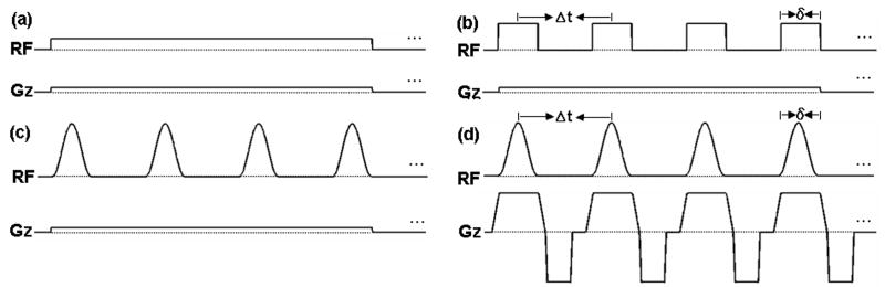
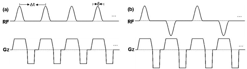
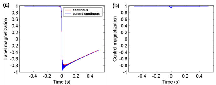
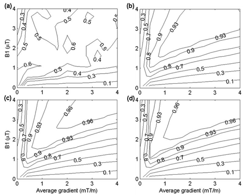
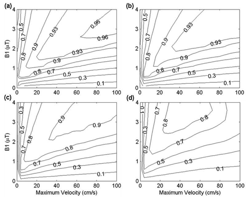
Continuous labeling by flow-driven adiabatic inversion is advantageous for arterial spin labeling (ASL) perfusion studies, but details of the implementation, including inefficiency, magnetization transfer, and limited support for continuous-mode operation on clinical scanners, have restricted the benefits of this approach. Here a new approach to continuous labeling that employs rapidly repeated gradient and radio frequency (RF) pulses to achieve continuous labeling with high efficiency is characterized. The theoretical underpinnings, numerical simulations, and in vivo implementation of this pulsed continuous ASL (PCASL) method are described. In vivo PCASL labeling efficiency of 96% relative to continuous labeling with comparable labeling parameters far exceeded the 33% duty cycle of the PCASL RF pulses. Imaging at 3T with body coil transmission was readily achieved. This technique should help to realize the benefits of continuous labeling in clinical imagers.

Figure 1

Different potential RF and gradient patterns for continuous labeling. (a) constant RF pulse, constant gradient. (b) Rectangular RF pulse train, constant gradient. (c) Hanning RF pulse train, constant gradient. (d) Hanning RF pulse train, variable gradient with strong gradient during RF pulses.

Figure 2

Suppression of aliased labeling planes with a stronger gradient during the RF pulse. When a constant gradient of 1mT/m is used, (a), many aliased labeling plans (solid vertical lines) are within the excitation profile of an individual RF pulse (dashed curve). When the gradient during the RF pulse is increased to 9 mT/m, without changing the average gradient, the primary labeling plane is unaffected (solid vertical line) but the aliased labeling plans, (vertical dashed lines) are suppressed because they fall outside the narrower excitation profile of the RF pulses (dashed curve). A pulse repetition time, Δt, of 1500 μs was used in this simulation.

Figure 3

The proposed pulsed-continuous ASL sequence: (a) the labeling pulse sequence with B1_ave ≠ 0, G_ave ≠ 0, (b) the control pulse sequence with B1_ave = 0, G_ave = 0.

Figure 4

Time courses of longitudinal magnetization of spins flowing across the labeling plane at t = 0. (a) during the label for PCASL (overlaid with continuous ASL with same average gradient and average B₁ amplitude); (b) during the control for PCASL from the numerical simulation of the Bloch equations.

Figure 5

Simulated inversion efficiency for laminar flow in a vessel as a function of RF field amplitude (μT) and average gradient amplitude (mT/m) at different ratio of G_max and G_ave: (a) G_max/G_ave = 2; (b) G_max/G_ave = 6; (c) G_max/G_ave = 9; (d) G_max/G_ave = 15. A constant maximum vessel velocity of 40.3 cm/s was assumed. An average gradient of 1 mT/m was used. This simulation is based on 500 μs Hanning shaped RF pulse and 1500 μs pulse repetition time. Contours are shown at efficiency values (0.1, 0.3, 0.5, 0.7, 0.8, 0.9, 0.93, 0.96) except efficiency values (0.4, 0.6) are added in (a) for clearer visibility of the efficiency distribution. The values shown were calculated using a correction for T₁ decay as well as velocity-weighting.

Figure 6

Simulated inversion efficiency for laminar flow in a vessel as a function of (a) the ratio G_max/G_ave. A constant maximum vessel velocity of 40.3 cm/s is assumed; (b) time gap between two RF pulses (Δt). A constant maximum vessel velocity of 40.3 cm/s was assumed, and the maximum gradient of 9 mT/m was used; (c) maximum velocity for control and label strategy in contrast with combined efficiency. A maximum gradient of 9 mT/m was used; (d) maximum velocity (cm/s) for different T₂ blood relaxation times: T₂ = 0.25 s; T₂ = 0.10 s while keeping T₁ as a constant 1.55 s; There is no noticeable efficiency difference between T₁ = 1.55 s and T₁ = 1.3 s for fixed T₂ of 0.25s. An average RF amplitude and gradient of 1.7 μT and 1 mT/m were used in the above simulations.

Figure 7

Simulated inversion efficiency for laminar flow in a vessel as a function of RF field amplitude (μT) and maximum velocity (cm/s) at (a) frequency offset = 0, (b) frequency offset = 1/(8Δt), (c) frequency offset = 1/(4Δt), (d) frequency offset = 3/(8Δt). A maximum gradient and average gradient of 0.9 and 0.1 were used. A constant maximum vessel velocity of 40.3 cm/s was assumed. Contours are shown at efficiency values (0.1, 0.3, 0.5, 0.7, 0.8, 0.9, 0.93, 0.96).

Figure 8

Single slice pulsed-continuous image of (a) label below – label above; (b) control below –control above; (c) control below – label below; (d) control above – label above; and 55% duty cycle continuous image of (e) label above – label below. The in-vivo experiment used an average B₁ amplitude of 1.7 μT, maximum gradient of 9 mT/m, and average gradient of 1 mT/m with 500 μs Hanning shaped RF pulse and 1500 μs pulse repetition time.

Figure 9

The mean signal difference when control and label are applied distal and proximal to the imaging plane as a function of frequency offset. Distance z from the labeling plane was converted to a frequency offset using γG_maxz. Proximal labeling produces a large signal difference, while distal labeling above the brain produces a very small signal difference.

Figure 10

Multi-slice perfusion difference images from a 3D whole-brain acquisition using the PCASL label and control strategy.

References

1. Detre JA, Leigh JS, Williams DS, Koretsky AP. Perfusion imaging. Magn Reson Med. 1992;23:37–45. - PubMed
1. Williams DS, Detre JA, Leigh JS, Koretsky AP. Magnetic resonance imaging of perfusion using spin inversion of arterial water. PNAS USA. 1992;89:212–216. - PMC - PubMed
1. Detre JA, Alsop DC. Perfusion magnetic resonance imaging with continuous arterial spin labeling: methods and clinical applications in the central nervous system. Eur J Radiol. 1999;30(2):115–124. - PubMed
1. Wolf RL, Detre JA. Clinical neuroimaging using arterial spin-labeled perfusion magnetic resonance imaging. Neurotherapeutics. 2007;4(3):346–359. - PMC - PubMed
1. Aguirre GK, Detre JA, Wang J. Perfusion fMRI for functional neuroimaging. Int Rev Neurobiol. 2005;66:213–236. - PubMed