Morphological appearance manifolds in computational anatomy: groupwise registration and morphological analysis

Abstract

Existing approaches to computational anatomy assume that a perfectly conforming diffeomorphism applied to an anatomy of interest captures its morphological characteristics relative to a template. However, the amount of biological variability in a groupwise analysis renders this task practically impossible, due to the nonexistence of a single template that matches all anatomies in an ensemble, even if such a template is constructed by group averaging procedures. Consequently, anatomical characteristics not captured by the transformation, and which are left out in the residual image, are lost permanently from subsequent analysis, if only properties of the transformation are examined. This paper extends our recent work [Makrogiannis, S., Verma, R., Davatzikos, C., 2007. Anatomical equivalence class: a computational anatomy framework using a lossless shape descriptor. IEEE Trans. Biomed. Imag. 26(4), 619-631] on characterizing subtle morphological variations via a lossless morphological descriptor that takes the residual into account along with the transformation. Since there are infinitely many [transformation, residual] pairs that reconstruct a given anatomy, we treat them as members of an Anatomical Equivalence Class (AEC), thereby forming a manifold embedded in the space spanned by [transformation, residual]. This paper develops a unique and optimal representation of each anatomy that is estimated from the corresponding AECs by solving a global optimization problem. This effectively determines the optimal template and transformation parameters for each individual anatomy, and eliminates respective confounding variation in the data. It, therefore, constitutes the second novelty, in that it represents a group-wise optimal registration strategy that individually adjusts the template and the smoothness of the transformation according to each anatomy. Experimental results support the superiority of our morphological analysis framework over conventional analysis, and demonstrate better diagnostic accuracy.

Figure 1

Effect of aggressive registration: (a) Subject; (b) Template; (c) Subject warped through a viscous fluid algorithm. Aggressively registering a bifolded sulcus to a single-folded sulcus creates very thin needle like structures, which are atypical of a human brain.

Figure 2

(a) Template; (b) Mean of 31 spatially normalized brains; (c) A representative subject; (d) Spatial normalization of (b) using HAMMER; (e) Corresponding residual. While crispness of the mean brain indicates reasonably good anatomical correspondence, there are still significant anatomical differences, which may be large enough to offset disease specific atrophy in a brain.

Figure 3

Manifold structure and intersubject comparisons based on Euclidean distance.

Figure 4

OMS versus CMD: (a) Randomly selecting CMDs (random parameter selection) reduces inter-group separation. Dots marked with arrows represent group means; (b) OMS results in optimal separation between the two groups.

Figure 5

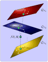
Approximation of AEC manifolds with hyperplanes. τ and λ may be two of the confounding factors invariance to which is sought, as explained later in Section 2.5.

Figure 6

Constructing AECs: Each subjects is normalized to Ω_T via intermediate templates at different smoothness levels of the warping transformations.

Figure 7

Intermediate templates aid registration: (a) Template of Fig 2(a); (b) Direct warping of Fig. 2(c); (c) Warping via an intermediate template.

Figure 8

Schematic illustration of tissue density maps (TDMs). Left column shows subjects of varying sizes, which are warped to the template given in middle column. When expansion takes place during warping of an individual shape to the template, the tissue density values are smaller (darker intensity), while in contraction the tissue density increases (brighter).

Figure 9

2D synthetic dataset – Templates T₁,…,T₁₂ simulating gray matter folds.

Figure 10

2D synthetic dataset – Dependence of residual on regularization λ: : See how registration deteriorates by changing the λ. (a) Subject; (b) Template; (c) Subject warped with the most aggressive transformation (small λ); (d) Subject warped with intermediate level aggression (intermediate λ); (e) Subject warped with very mild transformation (small λ).

Figure 11

2D synthetic dataset – Dependence of residual on template T: See how registration deteriorates by changing the template. (a) Subject; (b) Template T₁₂; (c) Subject warped to T₁₂; (d) Template T₁; (e) Subject warped to T₁.

Figure 12

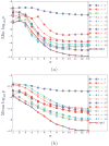
2D synthetic dataset – The effect of regularization parameter λ and smoothing σ on the performance of morphological descriptors without optimization, as depicted by minimum p-value plots based on the t-test for capturing significant group differences: (a) min log₁₀ p for LJD; (b) min log₁₀ p for Residual. For LJD, best performance is achieved for low regularization (λ = 3), whereas residual performs the best with intermediate regularization (λ = 27). Either cases correspond to large smoothing (σ = 13).

Figure 13

2D synthetic dataset – OMS versus CMDs for capturing significant group differences based on Hotelling’s T²-tests: (a) Minimum p values; (b) Mean of p-values after thresholding them to 10⁻². Optimization yields better performance with about an order of magnitude improvement in the p-values.

Figure 14

2D synthetic dataset – T²-test based log₁₀ p-value maps for 2D simulated data at σ = 13 thresholded to p ≤ 10⁻²: (a) CMD λ = 23; (b) OMS.

Figure 15

2D synthetic dataset – Hotelling’s T² test on CMD and OMS corresponding to the best case of Fig. 13, i.e., σ = 13, and λ = 23. Note that p-value maps are thresholded to p ≤ 10⁻⁴. Results are shown on a log₁₀-scale: (a) CMD with T₁; (b) CMD with T₂; (c) CMD with T₃; (d) OMS with T₁; (e) OMS with T₂; (f) OMS with T₃.

Figure 16

3D dataset: (a) A subject without atrophy; (b) With 10% simulated atrophy.

Figure 17

3D dataset – The effect of regularization parameter λ and smoothing σ on the performance of morphological descriptors without optimization, as depicted by minimum p-value plots based on the t-test for capturing significant group differences: (a) log J_hλ,τ; (b) R_hλ,τ. For log J_hλ,τ, best performance is achieved for low regularization (λ = 0), whereas R_hλ,τ performs the best for high regularization (λ = 7).

Figure 18

3D dataset – Hotelling’s T²-test based minimum p-value plots for CMDs and OMS. The performance of CMDs is highly dependent on λ. Optimization, on the other hand, removes this dependency as evident from the largely stable curve for OMS, which is also less sensitive to σ.

Figure 19

Atrophy maps as captured by CMD and OMS for the 3D dataset – T² test based p-value maps corresponding to the best results for each descriptor thresholded to p ≤ 10⁻⁵: (a) CMD λ = 7, σ = 4; (b) OMS with σ = 5.

Figure 20

Longitudinal dataset – Comparison between most conforming CMD (traditional approach) and OMS in terms of mean GM TDM in the ROI in the presence of atrophy: (a) Posterior Cingulate; (b) Hippocampus; (c) Superior temporal gyrus. Dotted lines represent the corresponding linear regression fits.

Figure 21

Longitudinal dataset – Comparison between CMD and OMS in terms of mean TDM in the ROI when no atrophy is present. Note that random fluctuations in traditional approach may contribute to incorrect estimation of the temporal profile. Dotted lines represent the corresponding linear regression fits.

Figure 22

Longitudinal dataset – Comparison between CMD (traditional approach) and OMS in terms of rate of atrophy: (a) CMD based regression map for TDM; (b) OMS based regression map for TDM. Note how OMS was able to eliminate growth falsely picked up by the traditional analysis, resulting in more accurate analysis.

References

1. Ashburner J, Friston K. Nonlinear spatial normalization using basis functions. Human Brain Mapping. 1999;7(4):254–266. - PMC - PubMed
1. Ashburner J, Friston KJ. Voxel-based morphometry – the methods. NeuroImage. 2000;11(6):805–821. - PubMed
1. Ashburner J, Hutton C, Frackowiak R, Johnsrude I, Price C, Friston K. Identifying global anatomical differences: deformation-based morphometry. Human Brain Mapping. 1998;6(6):348–357. - PMC - PubMed
1. Avants BB, Epstein CL, Gee JC. Geodesic image normalization and temporal parameterization in the space of diffeomorphisms. MIAR. 2006:9–16.
1. Baloch S, Verma R, Davatzikos C. An anatomical equivalence class based joint transformation-residual descriptor for morphological analysis. IPMI. 2007:594–606. - PubMed
Publication types