Cortical columnar organization is reconsidered in inferior temporal cortex

Abstract

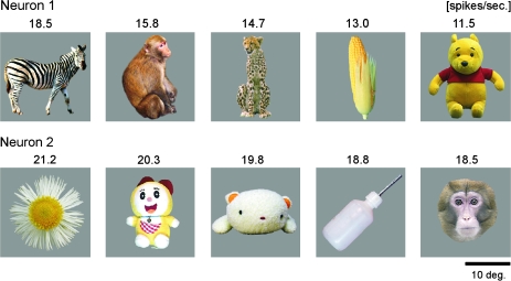
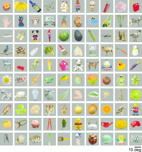
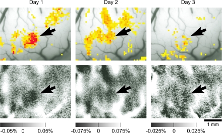
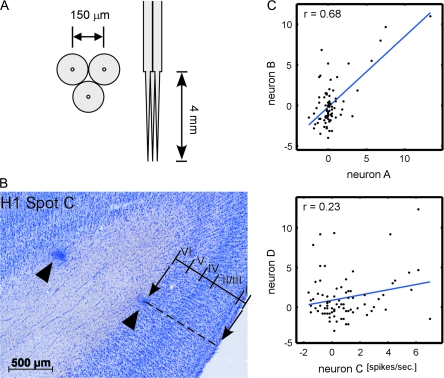
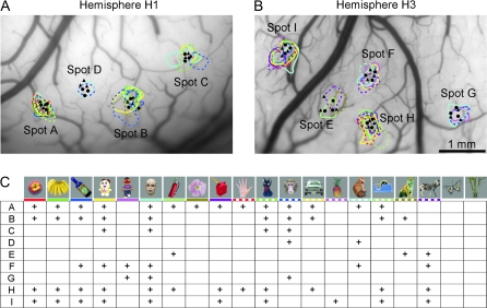
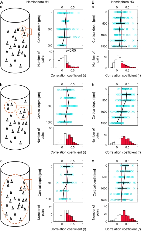
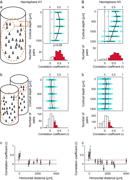
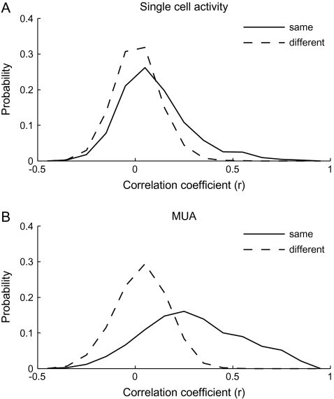
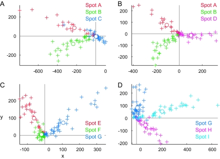
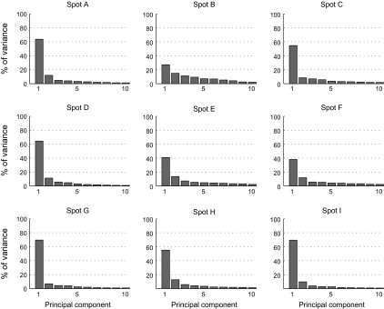
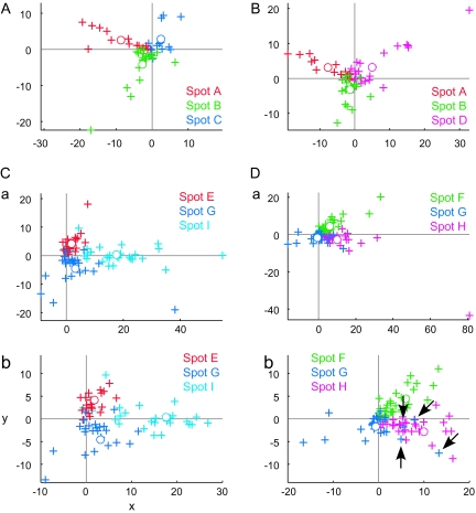
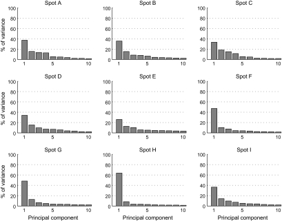
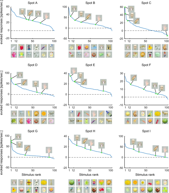
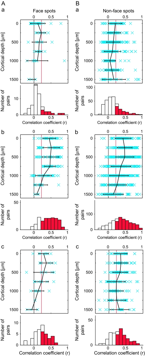
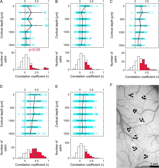
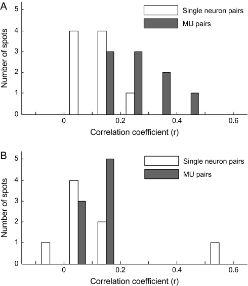
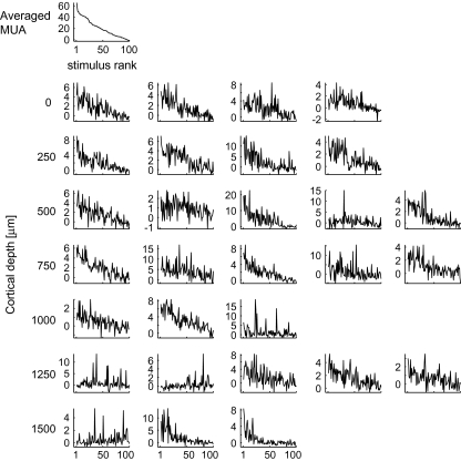
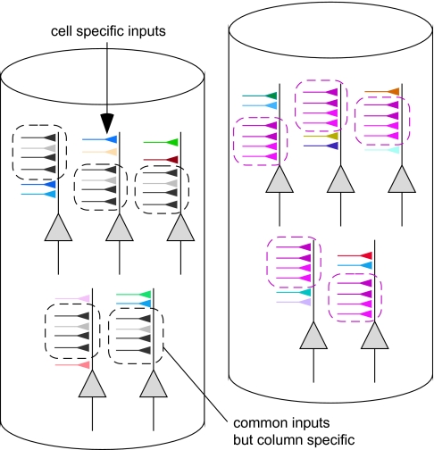
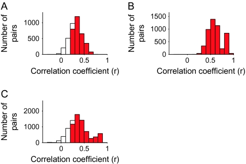
The object selectivity of nearby cells in inferior temporal (IT) cortex is often different. To elucidate the relationship between columnar organization in IT cortex and the variability among neurons with respect to object selectivity, we used optical imaging technique to locate columnar regions (activity spots) and systematically compared object selectivity of individual neurons within and across the spots. The object selectivity of a given cell in a spot was similar to that of the averaged cellular activity within the spot. However, there was not such similarity among different spots (>600 microm apart). We suggest that each cell is characterized by 1) a cell-specific response property that cause cell-to-cell variability in object selectivity and 2) one or potentially a few numbers of response properties common across the cells within a spot, which provide the basis for columnar organization in IT cortex. Furthermore, similarity in object selectivity among cells within a randomly chosen site was lower than that for a cell in an activity spot identified by optical imaging beforehand. We suggest that the cortex may be organized in a region where neurons with similar response properties were densely clustered and a region where neurons with similar response properties were sparsely clustered.

Figure 1.

A case showing that the top 5 object stimuli of 2 adjacent isolated neurons were completely different. Each row gives the top 5 visual stimuli for a neuron. For each neuron, these 5 stimuli elicited visual responses stronger than the other 95 object stimuli. The number at each picture indicates the evoked response elicited by the stimulus (spikes/s). These neurons were spaced 150 μm apart. The response similarity between these cells for 100 object stimuli, expressed as a correlation coefficient of evoked responses, was 0.22.

Figure 2.

One hundred object stimuli used for examination of object selectivity. The stimuli in the top 2 rows were also used in intrinsic signal imaging sessions.

Figure 3.

Reproducible responses of intrinsic signals to an object stimulus. Upper panels indicate regions in which the reflection increases elicited by the stimulus were significantly greater than the increases of reflection caused by spontaneous fluctuation. The highest significance level is denoted by red and the lowest by yellow where P < 0.05 (t-test). Lower panels indicate reflection changes of the cortex elicited by visual stimulus presentation (see Tsunoda et al. 2001 for details). Horizontal scales represent percent changes in reflection. The optical responses at the first, second, and third days are represented from left to right. The arrow indicates reproducible active spots. The stimulus that elicited the activation was the upper-left object image in Figure 2.

Figure 4.

Analysis of the stimulus selectivity of neurons. (A) Design of a bundle of tungsten electrodes used in this study. Left and right pictures show the bottom and side view of the electrode bundle. Electrode-to-electrode distance was designed to be about 150 μm at the tip. The exact locations of the electrodes are indicated in Figure 5. (B) A histological section of the region including one spot obtained after all the extracellular recording sessions were completed. Two arrowheads indicate the sites of electrocoagulation made at the last penetration of the spot. Based on the depths of the coagulation and borders between the cortical layers, we evaluated the relationship between depth and cortical layers (see Table 1). (C) Representative scattergrams indicating similarity in object selectivity of 2 isolated neurons. In each figure, horizontal and vertical axes indicate evoked responses of 2 neurons, and each symbol in the scattergrams indicates an object image. The values of correlation coefficient in the upper and lower panels were 0.68 and 0.23, respectively. These values were statistically significant (P < 0.05, number of object images = 80).

Figure 5.

Activity spots revealed by intrinsic signal imaging. (A, B) Activity spots in H1 (A) and H3 (B) were demarcated by colored contours. Penetration sites of electrodes are indicated by a filled circle (first-day penetration) and triangle (second-day penetration). (C) Optical response patterns of individual spots to 20 stimuli used in intrinsic signal imaging. Each column represents presence (cross) or absence (no symbol) of responses to the stimulus indicated on the top. Rows A–I correspond to spots A–I. The colored horizontal bar under the stimuli is to correlate a stimulus to the activity spots elicited by the stimulus in (A) and (B): The same color is used for the bar under each stimulus and for the contour of the activity spots elicited by the stimulus. Reliability of intrinsic signal imaging for an individual activity spot was assessed by calculating correlation coefficients between optical responses of the spot and averaged MUAs recorded from the spot for 20 stimuli used for intrinsic signal imaging. The resulting values of the correlation coefficient were 0.85, 0.43, 0.59, and 0.75 for spots A, B, C, and D obtained from H1 and 0.57, 0.50, 0.80, 0.29, and 0.63 for spots E, F, G, H, and I obtained from H3. Because the significant correlation coefficient value was 0.4 for 20 object images (P < 0.05), intrinsic signal imaging reliably revealed activity spots except for spot H.

Figure 6.

Similarity in stimulus selectivity between single isolated cells (Aa, Ba), MUs (Ab, Bb), and between single isolated cells and averaged MUs (Ac, Bc). (Aa, Ba) The values of correlation coefficient (r) between evoked responses to 80 object stimuli were calculated for isolated single-neuron pairs recorded at the same depth as schematically drawn in (Aa) (inset). Upper panels in (Aa) and (Bb) represent relationships between the r values (horizontal axes) and depth of the recording sites of the pairs (vertical axes). The mean (black) and the r values of individual pairs (crosses in blue) are indicated. Error bars represent SD. The red vertical line in each panel indicates the statistically significant threshold (r = 0.22, P < 0.05 for 80 stimuli). Lower histograms in (Aa) and (Ba) represent the distributions of the pairs with respect to their r values. The number of pairs was the sum across the depth. The columns indicated in red represent the number of pairs with significant correlation. The mean value of correlation coefficient (r) and the proportion of pairs with significant correlation were 0.11 and 21.2%, respectively, in (Aa) and 0.15 and 28.5%, respectively, in (Bb). (Ab, Bb) Correlation between evoked responses to 80 object stimuli were calculated as in (Aa) and (Ba) for the MU pairs recorded at the same depths as schematically drawn in (Ab, inset). Conventions in (Ab) and (Bb) are the same as (Aa) and (Ba). In the lower histograms, the mean value of correlation coefficient (r) and the proportion of pairs with significant correlation were 0.23 and 51.9%, respectively, in (Ab) and 0.28 and 60.0%, respectively, in (Bb). (Ac, Bc) Correlation coefficients were calculated between evoked responses to 80 object stimuli of isolated single neurons and those of evoked responses of averaged MUs as schematically drawn in (Ac) left. Conventions in (Ac) and (Bc) are the same as (Aa) and (Ba). In the lower histograms, the mean value of correlation coefficient (r) and the proportion of pairs with significant correlation were 0.18% and 40.0%, respectively, in (Ac) and 0.32% and 65.7%, respectively, in (Bc); (A) are the results obtained from spots A–D (H1), and (B) are from spots E–I (H3).

Figure 7.

Similarity in stimulus selectivity within a spot and across 2 spots. (Aa, Ba) The values of correlation coefficient were calculated between evoked responses to 80 object stimuli of averaged MUs and those of evoked responses of individual MUs within the same spots, as schematically drawn in (Aa) left. Please note that an MUA was excluded from the averaged MU when correlation coefficient was calculated between this MU and the averaged MU. Conventions in (Aa) and (Ba) are the same as Figure 6(Aa,Ba). (Ab, Bb) Correlation coefficients were calculated between evoked responses to 80 object stimuli of averaged MUs and those of evoked responses of individual MUs in the other spots, as schematically drawn in (Ab) left. Conventions in (Ab) and (Bb) are the same as Figure 6(Aa,Bb). (Ac, Bc) The values of the correlation coefficients shown in (Aa), (Ba), (Ab), and (Bb) are plotted against distances between spots. To distinguish values obtained from the MUs and averaged MUs of the same spots, the points were slightly displaced from distance 0. The values of correlation coefficients were averaged across the depth. The mean value and SD are plotted. The horizontal red lines indicate statistical significant levels (P < 0.05, r = 0.22). The distances were measured from the surface images and recording sites (Fig. 5A,B).

Figure 8.

Demonstration that common response properties existed for the cells within an activity spot but did not for cells across the activity spots. (A) Distributions of single-neuron pairs with respect to the values of the correlation coefficients between evoked responses to 80 stimuli of the cells in each pair. The solid line represents the distribution of pairs where cells were chosen from the same spots and the dotted line represents the distribution of pairs where cells were chosen from different spots. (B) Distributions of MU pairs with respect to the values of the correlation coefficients between evoked responses to 80 stimuli of the MUs in each pair. As in (A), the solid line represents the distribution of pairs of MUs from the same spots and the dotted line represents the distribution of pairs of MUs from different spots. Please note that the constituent members of a pair were chosen regardless to the depth that they were recorded from. Thus, in contrast to Figure 6, the members of pairs do not necessarily located close to each other even they are recorded from the same spot.

Figure 9.

Distribution of MUs in the stimulus space indicating that MUs of each spots are clustered together. MUs and averaged MUs of activity spots are plotted on the stimulus space, that is, 100 dimensional space in which each dimension represents responses (spikes/s) to one of the 100 object images. We chose the 2D plane that includes points representing responses of averaged MUs of 3 spots to demonstrate clustering MUs of the 3 spots in each figure. Crosses, responses of MUs projected on the 2D plane. Open circles, responses of averaged MUs. Different colors indicate different spots. (A, B) Represent MUs of the spots in hemisphere H1. (C, D) Represent MUs of the spots in hemisphere H3.

Figure 10.

Contribution of each component in PCA of MUs of each spot in the stimulus space. Each figure represents the result of the analysis applied for one of the activity spots. Horizontal axes represent rank-ordered principal components. Only first 10 components are indicated. Vertical axes represent proportion of variance explained by each principal component.

Figure 11.

Distribution of single cells in the stimulus space. Responses of single cells (crosses) and average of single cells (open circles) are plotted on the stimulus space as in the case of MUs in Figure 9.We chose the 2D plane that includes points representing responses of average of single-cell responses of 3 spots. Different colors indicate different spots. (A, B) represent single cells of the spots in hemisphere H1. (Ca, Da) represent single cells of the spots in hemisphere H3. Some cells had very large responses compared with other cells, and it is difficult to capture overall patterns of distribution; spots in hemisphere H3 were plotted in magnified view (Cb, Db) as well.

Figure 12.

Contribution of each component in PCA of single cells of each spot in the stimulus space. Conventions are the same as in Figure 10.

Figure 13.

Rank-ordered stimulus responses of MUs (spikes/s) for each activity spot. Responses to faces and hands of human and monkey are indicated in each figure. The pictures below each figure represent top 12 object stimuli that are arranged in descending order from left to right. The upper row indicates the best to the 6th best images and the lower row indicates the 7th to the 12th images.

Figure 14.

Comparison between face-selective spots and the other spots for similarity in stimulus selectivity. The results for spots C and G are represented in (A), and the results for the other spots are represented in (B). The other conventions are the same as in Figure 6. In (Aa, Ba), the values of the correlation coefficient were 0.12 ± 0.21 (mean ± SD, n = 55) and 0.13 ± 0.22 (mean ± SD, n = 323), respectively. The proportions of pairs that showed significant correlation were 18.2% and 27.2% for (Aa) and (Ba), respectively. In (Ab, Bb), the values of the correlation coefficient were 0.42 ± 0.24 (mean ± SD, n = 163) and 0.37 ± 0.29 (mean ± SD, n = 567), respectively. The proportions of pairs that showed significant correlation were 76.1% and 68.4% for (Ab) and (Bb), respectively. In (Ac, Bc), the values of the correlation coefficient were 0.22 ± 0.21 (mean ± SD, n = 40) and 0.29 ± 0.23 (mean ± SD, n = 178), respectively. The proportions of pairs that showed significant correlation were 47.5% and 59.0% for (Ac) and (Bc), respectively.

Figure 15.

Similarity in stimulus selectivity between single isolated cells, MUs, and between single isolated cells and averaged MUs in hemisphere H2, where recording sites were randomly chosen without the guidance of intrinsic signal imaging. (A, B, C) correspond to Figures 6(Aa,Ba), (Ab,Bb), and (Ac,Bc), respectively. Conventions are the same as in Figure 6. (D, E) correspond to Figures 7(Aa,Ba) and (Ab,Bb), respectively. Conventions are the same as in Figure 7. (F) represents recording sites from hemisphere H2. Density of recordings within individual sites, and site-to-site distances, was adjusted nearly the same as in H1 and H3.

Figure 16.

Relationship of object selectivity between single-neuron pairs and MU pairs for the spots identified by intrinsic signal imaging (A) and for the randomly chosen sites (B). The mean value of correlation coefficient (r) was calculated separately for each spot, and distribution of spots was plotted against the mean values of correlation coefficient. Total number of spots was 9 (4 spots from H1 and 5 spots from H3) for activity spots and 8 for randomly chosen sites.

Figure 17.

Tuning curves of the individual cells in a representative spot and the tuning curve of averaged MUs of the spot. The graph at the left upper corner represents the tuning curve of averaged MUs and the rests represent tuning curves of single cells at different depths. Depth of cells in each row is indicated at the left. Horizontal axes are rank ordered according to the magnitude of evoked responses of averaged MUs to the 100 object stimuli in descending order. Vertical axes represent mean firing rate (spikes/s).

Figure 18.

Schematic drawing of cell-specific inputs and inputs common among cells within a spot. Two columns are represented. The synaptic inputs demarcated by broken lines represent common inputs. These inputs are different from column to column. In this figure, the differences in common inputs for the 2 columns are indicated by the color of the inputs (left column, gray and right column, pink). Other inputs represent cell-specific synaptic inputs. We consider that these differences in synaptic inputs generate common and cell-specific response properties.

Figure 19.

Demonstration showing increase of similarity in object selectivity by averaging activities of single cells. In each hemisphere, isolated cells were divided into 2 groups with equal number, and each group is averaged. A correlation coefficient was calculated between the evoked responses to 80 object images of these 2 averaged groups. Isolated cells were divided into 2 groups in 1000 different combinations, and resulting correlation coefficients were plotted in frequency distribution against the values of correlation coefficients. (A, B, C) were the frequency distribution obtained from hemispheres H1, H3, and H2, respectively. The mean and SD of the correlation coefficients were 0.35 ± 0.11, 0.59 ± 0.16, and 0.41 ± 0.20 for H1, H3, and H2, respectively. The column in red represents the pairs with significant correlation (P < 0.05, r = 0.22).

References

1. Albright TD, Desimone R, Gross CG. Columnar organization of directionally selective cells in visual area MT of the macaque. J Neurophysiol. 1984;51:16–31. - PubMed
1. Arieli A, Grinvald A, Slovin H. Dural substitute for long-term imaging of cortical activity in behaving monkeys and its clinical implications. J Neurosci Methods. 2002;114:119–133. - PubMed
1. Baker C, Knouf N, Wald L, Fischl B, Kwang K, Benner T, Kanwisher N. Functional selectivity of human extrastriate visual cortex at high resolution. J Vis. 2004;4:88–88.
1. Cheng K, Waggoner RA, Tanaka K. Human ocular dominance columns as revealed by high-field functional magnetic resonance imaging. Neuron. 2001;32:359–374. - PubMed
1. Desimone R, Albright TD, Gross CG, Bruce C. Stimulus-selective properties of inferior temporal neurons in the macaque. J Neurosci. 1984;4:2051–2062. - PMC - PubMed
Publication types