Development of a mathematical model for predicting electrically elicited quadriceps femoris muscle forces during isovelocity knee joint motion

Abstract

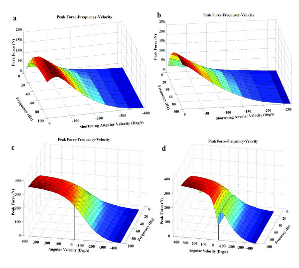
Background: Direct electrical activation of skeletal muscles of patients with upper motor neuron lesions can restore functional movements, such as standing or walking. Because responses to electrical stimulation are highly nonlinear and time varying, accurate control of muscles to produce functional movements is very difficult. Accurate and predictive mathematical models can facilitate the design of stimulation patterns and control strategies that will produce the desired force and motion. In the present study, we build upon our previous isometric model to capture the effects of constant angular velocity on the forces produced during electrically elicited concentric contractions of healthy human quadriceps femoris muscle. Modelling the isovelocity condition is important because it will enable us to understand how our model behaves under the relatively simple condition of constant velocity and will enable us to better understand the interactions of muscle length, limb velocity, and stimulation pattern on the force produced by the muscle.

Methods: An additional term was introduced into our previous isometric model to predict the force responses during constant velocity limb motion. Ten healthy subjects were recruited for the study. Using a KinCom dynamometer, isometric and isovelocity force data were collected from the human quadriceps femoris muscle in response to a wide range of stimulation frequencies and patterns. % error, linear regression trend lines, and paired t-tests were used to test how well the model predicted the experimental forces. In addition, sensitivity analysis was performed using Fourier Amplitude Sensitivity Test to obtain a measure of the sensitivity of our model's output to changes in model parameters.

Results: Percentage RMS errors between modelled and experimental forces determined for each subject at each stimulation pattern and velocity showed that the errors were in general less than 20%. The coefficients of determination between the measured and predicted forces show that the model accounted for approximately 86% and approximately 85% of the variances in the measured force-time integrals and peak forces, respectively.

Conclusion: The range of predictive abilities of the isovelocity model in response to changes in muscle length, velocity, and stimulation frequency for each individual make it ideal for dynamic applications like FES cycling.

Figure 1

Schematic representation of the three stimulation patterns used. Bottom train (CFT50) is a constant-frequency train with all interpulse intervals equal to 50 ms; middle train (VFT50) is a variable-frequency train with an initial doublet of 5 ms and remaining pulses equally spaced by 50 ms; and top train (DFT50) is a doublet-frequency train with 5-ms doublets separated by interdoublet interval of 50 ms. Each train's name is based on the duration of the longest interpulse interval within that train. Each train has a maximum of 50 pulses (not shown in figure) and a pulse width of 600 μs.

Figure 2

A) Schematic representation of a Hill-type model used for modeling the muscle's response to electrical stimulation. The muscle modeled as a linear series spring, linear damper, and a motor. The parallel elastic element was neglected because for the range of motion studied in the current study the passive forces are smaller than the active force. k_s is the spring constant of the series element, b is the damping coefficient of the damper, and V is the velocity of the motor. The force exerted by the spring and damper are k_sx and $b(\dot{y}-\dot{x})$, respectively. The velocity of the motor is given by $V=\dot{y}-\dot{z}=B\frac{C_N}{K_M+C_N}$, where B is the constant of proportionality (see text for details). B) Schematic representation of the leg modeled as single rigid body segment (tibia) when subjected to stimulation under isovelocity conditions. In the isovelocity mode, the KinCom arm moves the tibia at a constant angular velocity ($\dot{\theta }$ = constant). θ is the knee flexion angle. L is the distance from the knee joint center to the center of the force transducer placed above the ankle and l is the distance from the knee center of rotation to the center of mass of the tibia. T_stim is the torque due to stimulation, F_EXT is the force measured by the KinCom dynamometer, mg is the weight of the tibia-foot complex (foot not shown in figure), and H is the resistance moment to knee extension due to visco-elasticity of the musculotendon complex of the knee joint.

Figure 3

Overview of the distribution of subjects used for model development and validation. See text for details about the characteristics of the parameterizing and testing trains.

Figure 4

Flowchart of the steps involved in the parameter identification during the model development phase. Please note, during the model validation phase the steps involved in the parameter identification are identical to those outlined in the above flow chart, except that parameters M, V₁, and V₂ will be identified at the velocity determined from the model development phase.

Figure 5

Experimental, fitted, and predicted forces in response to the VFT20-VFT80 train combination from a typical subject at different shortening velocities during the model development phase. For each row, the shaded panel represents the fittings of the VFT20-VFT80 experimental data to that velocity, while the non-shaded panels represent model predictions to the other three velocities. For example, the shaded panel (f) at -75°/s represents the fitting of the isovelocity model to the experimental forces data, while the non-shaded panels (e), (g), and (h) are the predictions of the model at -25°/s, -125°/s, and -200°/s, respectively. These data were used to determine the best velocity to identify the parameters V₁ and V₂. RMS Force (N) errors between measured and modeled force data in response to the VFT20-VFT80 train are presented in each panel. It should be noted that the experimental data in the figure are means of two trails.

Figure 6

Bar graphs of FAST first order sensitivity index of the seven model parameters under isometric conditions at a knee flexion angle of 90° and the four isovelocity conditions of 25°/s, 75°/s, 125°/s, and 200°/s. Higher the value of the sensitivity index of a parameter, greater is sensitivity of the model output (force-time integral) to changes in that model parameter.

Figure 7

Experimental, fitted, and predicted forces from a typical subject's quadriceps femoris muscle at different constant shortening speeds during the model validation phase. (a): Fitting of the experimental force data in response to VFT20-VFT80 train combination at 40° of knee flexion (isometric) to determine the values of a, b, A₄₀, τ₁, τ₂, and K_m (b): Fitting the experimental force data in response to VFT20-VFT80 train combination at 200°/s to determine the value of V₁. (c)-(e): Comparison of experimental and predicted forces in response to CFT10, CFT50, and CFT100 (panel c), VFT30, VFT50, and VFT100 (panel d), and DFT30, DFT70, and DFT100 (panel e) at a shortening speed of -25°/s. (f)-(n): Comparison of experimental and predicted forces in response to the above stimulation trains at -75°/s (panels f-h), -125°/s (panels i-k), and -200°/s (panels l-n). The isovelocity model parameter values for this subject were: a = -0.00165, b = -0.0662, A₄₀ = 3.42686, τ₁ = 30.69527, τ₂ = 91.07621, K_m = 0.23564, R₀ = 2, τ_c = 20, and V₁ = 0.00074.

Figure 8

Bar graphs of comparisons between the mean (+ standard error) experimental and predicted peak forces (a, c, e, and g) and force-time integrals (b, d, f, and h) of six subjects used for validation of the isovelocity model. Responses to CFTs with interpulse intervals of 10, 30, 50, 70, and 100 ms (C10, C30, C50, C70, C100), responses to VFTs with interpulse intervals of 20, 30, 50, 70, 80, 100 ms (V20, V30, V50, V70, V80, and V100), and responses to DFTs with interpulse intervals of 30, 50, 70, 100 ms (D30, D50, D70, and D100) at shortening velocities of -25°/s (a and b), -75°/s (c and d), -125°/s (e and f), and -200°/s (g and h) are shown. * = p ≤ 0.05 (see text for details). It should be noted that the experimental data in the figure are means of two trails. Also, note the difference in scaling of the y-axis between panels a, b, c, and d and panels e, f, g, and h.

Figure 9

Plots of force-time integrals (a, c, e, and g) and peak forces (b, d, f, and h) of experimental versus predicted forces for six subjects at shortening velocities of -25°/s (a and b), -75°/s (c and d), -125°/s (e and f), and -200°/s (g and h). Solid lines in (a)-(e) are the identity lines. R² values were calculated.

Figure 10

Variations in the force velocity relationship with stimulation frequency, number of pulses, and the length where the stimulation is initiated. (a) The modeled peak force versus velocity curve does not follow the hyperbolic relationship when the stimulation train is initiated at 90° of knee flexion and is terminated when either 15° of knee flexion is reached or when 50 pulses were delivered. (b) Change in force velocity curve when the stimulation train is initiated at a knee flexion angle of 60°, the optimal muscle length for this subject. (c) Shortening contractions (negative angular velocities) and lengthening contractions (positive angular velocities) were performed when the leg was moving between 90° to 15° of knee flexion and the stimulation was applied throughout the range of motion. The model accurately captures the shape during shortening and lengthening contractions. The isomeric peak force was plotted at 60° of knee flexion. (d) The plot when the leg moves through the same shortening range (90° to 15°) and lengthening range (15° to 90°) as in c, except that the maximum number of pulses were now limited to 50 and the isometric peak force was considered at 15° of knee flexion to ensure a continuity in the force-velocity curves.

References

1. Bajd T, Kralj A, Turk R, Benko H, Sega J. Use of functional electrical stimulation in the rehabilitation of patients with incomplete spinal cord injuries. J Biomed Eng. 1989;11:96–102. doi: 10.1016/0141-5425(89)90115-5. - DOI - PubMed
1. Binder-Macleod S, Kesar T. Catchlike property of skeletal muscle: recent findings and clinical implications. Muscle Nerve. 2005;31:681–693. doi: 10.1002/mus.20290. - DOI - PubMed
1. Kebaetse MB, Binder-Macleod SA. Strategies that improve human skeletal muscle performance during repetitive, non-isometric contractions. Pflugers Arch. 2004;448:525–532. doi: 10.1007/s00424-004-1279-0. - DOI - PubMed
1. Garland SJ, Griffin L. Motor unit double discharges: statistical anomaly or functional entity? Can J Appl Physiol. 1999;24:113–130. - PubMed
1. Ding J, Wexler AS, Binder-Macleod SA. A mathematical model that predicts the force-frequency relationship of human skeletal muscle. Muscle Nerve. 2002;26:477–485. doi: 10.1002/mus.10198. - DOI - PubMed
Publication types