Adaptive-optics optical coherence tomography for high-resolution and high-speed 3D retinal in vivo imaging

Abstract

We have combined Fourier-domain optical coherence tomography (FD-OCT) with a closed-loop adaptive optics (AO) system using a Hartmann-Shack wavefront sensor and a bimorph deformable mirror. The adaptive optics system measures and corrects the wavefront aberration of the human eye for improved lateral resolution (~4 μm) of retinal images, while maintaining the high axial resolution (~6 μm) of stand alone OCT. The AO-OCT instrument enables the three-dimensional (3D) visualization of different retinal structures in vivo with high 3D resolution (4×4×6 μm). Using this system, we have demonstrated the ability to image microscopic blood vessels and the cone photoreceptor mosaic.

Fig. 1

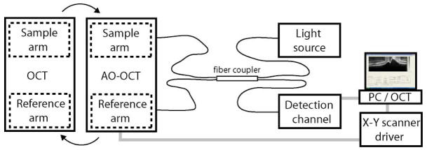
Schematic of the OCT engine used in our experiments. Black lines - fiber connections; gray lines - electrical connections. Two separate sample and reference arms permit switching between OCT and AO-OCT imaging systems. The splitting ratio of the fiber coupler was 80/20 (reference/sample)

Fig. 2

Schematic of the AO - control system used in our experiments. Black lines represent light paths and gray denotes electrical connections.

Fig. 3

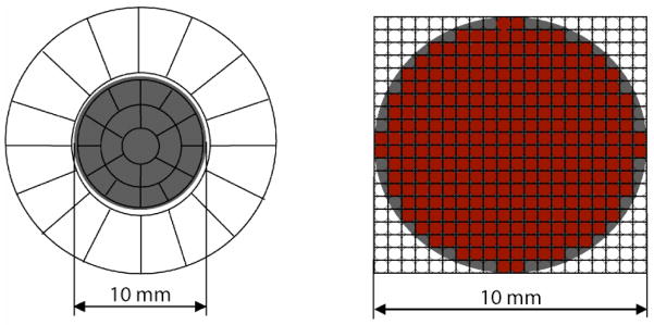
Actuator geometry for the 35-element AOptix DM (left) and Hartmann-Shack 400-lenslet configuration (right). The gray area corresponds to an image of a 7 mm eye pupil diameter. Note different scales for DM and lenslet array. Red circles on the right image indicate “active” spots used for wavefront calculation.

Fig. 4

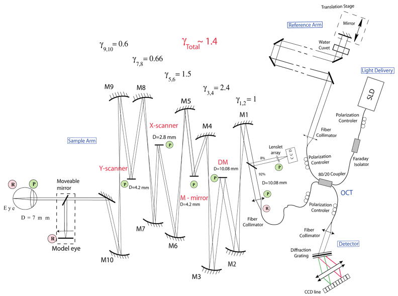
Schematic of UC Davis AO – OCT experimental setup constructed on a standard laboratory optical table occupying 1×1 m. The reference arm length has been shortened on the illustration for simplification. Key: γ - magnification, D - diameter, DM – deformable mirror; M1-M10 – spherical mirrors, P – pupil plane, R - retinal plane.

Fig. 5

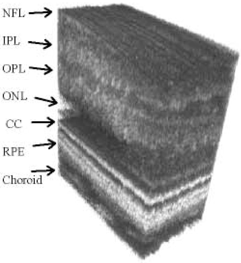
High-resolution B-scan of retinal structures acquired with our OCT instrument scanning 6 mm lateral range (4000 A-scans). We have identified the following retinal layers based on comparison with the literature: Nerve Fiber Layer (NFL), Ganglion Cell Layer (GCL), Inner Plexiform Layer (IPL), Inner Nuclear Layer (INL), Outer Plexiform Layer (OPL), Fibers of Henle with Outer Nuclear Layer (ONL), Inner Segment Layer (ISL), Outer Segment Layer (OSL), Retinal Pigment Epithelium (RPE), Choriocapillaris and Choroid. The Outer Limiting Membrane (sometimes called External Limiting Membrane), Connecting Cilia and Verhoeff’s Membrane may also be seen. The Fibers of Henle cannot be distinguished from the ONL in this image. The Inner Limiting Membrane and Bruch’s Membrane are also not visible on this image but have been confirmed using the same OCT system for imaging diseased retinas. The green rectangle denotes the scanning range of 500 μm used by our AO-OCT system when imaging at an eccentricity of 4 deg temporal retina (TR).

Fig. 6

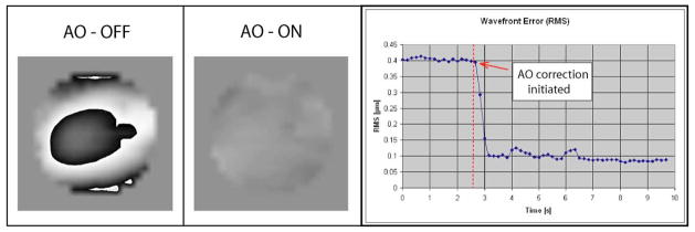
The ocular wavefront measured by H-S wavefront sensor before (left) and after (center) AO-correction. Left and center images present the reconstructed PSF for these wavefronts. Right plot shows total wavefront RMS error over time as measured by the H-S wavefront sensor before and during correction. The RMS error was corrected at a rate of 25 Hz but is displayed at rate of 6 Hz.

Fig. 7

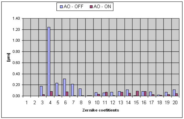
Reconstructed Zernike coefficients measured before (blue) and during (red) AO correction. Numbers correspond to the following Zernike coefficients: second-order aberrations: 3,5 – astigmatism, 4 – defocus; third-order aberrations: 6,9 – trefoil, 7,8 – coma; fourth- order aberrations: 10,14 – tetrafoil, 11,13 – 2nd astigmatism, 12 – spherical aberrations; fifth-order aberrations 15–20

Fig. 8

(1.34 MB) Real-time movie of retina acquired with AO-OCT during initiation of AO correction. The image covers 1×1 mm (1000 A-scans/Frame). (5.15 MB version)

Fig. 9

In vivo OCT images of AO-corrected retinal structures with axial intensity profiles for seven different focusing positions (both in logarithmic scale). The narrow depth of focus manifests itself by increases in intensity of the structures at the beam focus. All images have been acquired over 500 μm lateral distance. The effect of shifting the plane of focus on B-scans is illustrated. A white arrow marks the position of the focus plane on retinal structures. The image covers 0.5 × 1mm, comprising 512 × 500 pixels of original data (depth × width). The vertical axes are scaled identically for all intensity profiles and range from −65 dB (top limit) to −100 dB (lower limit) in sample reflectivity.

Fig. 10

(1.3 MB) Movie presenting 3D visualization of microscopic retinal structure reconstructed from 200 laterally displaced B-scans (with 500 A-scans/B-scan) covering 400×200×800 μm (lateral × lateral × depth). The focus position was set on the upper retinal layers (+0.5 diopter). (14.3 MB version)

Fig. 11

(0.98 MB) Movie sequence of the C-scan (flat illumination) reconstructed from the 3D volume 1000×100×512 voxels (lateral × lateral × depth). The white line on the B-scan (right) corresponds to the position of the reconstructed C-scan (left). C-scan image size: 1×1mm (3×3 deg) (lateral sampling = 1 μm between A-scan and 10 μm between B-scans), eccentricity of 6 deg nasal retina. (7.36 MB version)

Fig. 12

B-scans taken from the volumetric data (left) with corresponding 1D averaged power spectrum (center) (calculated from C-scans). The data have been acquired at two different retinal eccentricities, 2 deg (upper) and 4 deg (lower) temporal retina (TR). Central graph shows intensity encoded averaged 1D power spectrum calculated at each retinal depth revealing the presence of regular structures in both plexiform layers (capillaris), photoreceptor layers and choriocapillaris and choroid. Right graph shows 1D power spectrum at connecting cilia for the two retinal locations. Arrows indicate the spatial frequency corresponding to the peaks in the power spectra. The values of 33 cyc/deg and 50 cyc/deg correspond to spacings of 10 μm and 6.7 μm respectively, between imaged structures.

References

-
- Fercher AF, Hitzenberger CK, Kamp G, Elzaiat Y. Measurement of intraocular distances by backscattering spectral interferometry. Opt Commun. 1995;117:43–48.
- Wojtkowski M, Leitgeb R, Kowalczyk A, Bajraszewski T, Fercher AF. In Vivo human retinal imaging by fourier domain optical coherence tomography. J Biomed Opt. 2002;7:457–463. - PubMed
- Nassif NA, Cense B, Park BH, Pierce MC, Yun SH, Bouma BE, Tearney GJ, Chen TC, de Boer JF. In vivo high-resolution video-rate spectral-domain optical coherence tomography of the human retina and optic nerve. Opt Express. 2004. pp. 367–376. http://www.opticsexpress.org/abstract.cfm?URI=OPEX-12-3-367. - PubMed
- de Boer JF, Cense B, Park BH, Pierce MC, Tearney GJ, Bouma BE. Improved signal-to-noise ratio in spectral-domain compared with time-domain optical coherence tomography. Opt Lett. 2003;28:2067–2069. - PubMed
Grants and funding
LinkOut - more resources
Full Text Sources
Other Literature Sources