A robust automated system elucidates mouse home cage behavioral structure

Abstract

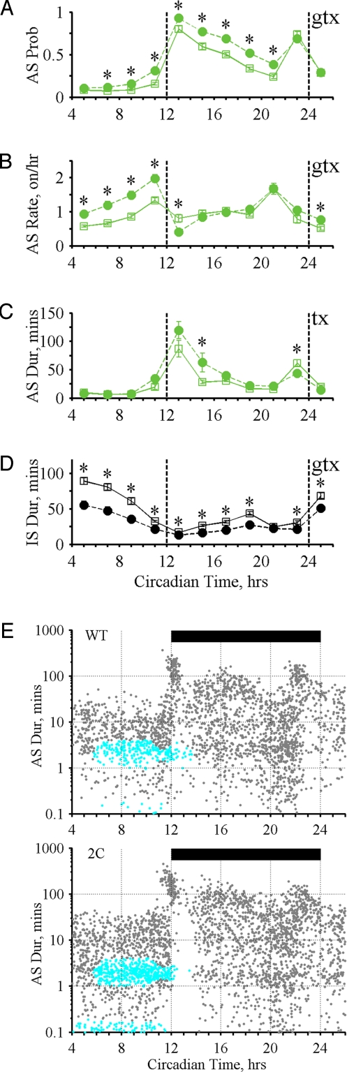
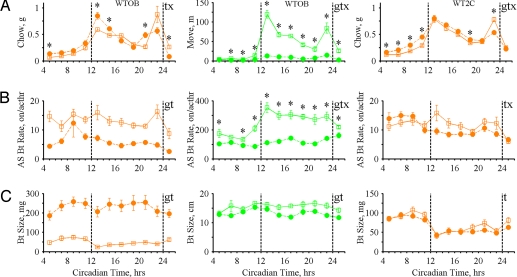
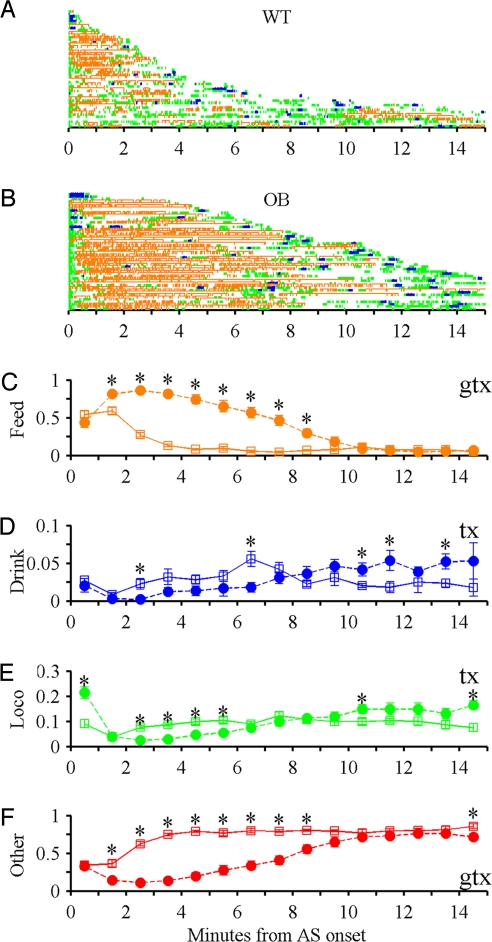
Patterns of behavior exhibited by mice in their home cages reflect the function and interaction of numerous behavioral and physiological systems. Detailed assessment of these patterns thus has the potential to provide a powerful tool for understanding basic aspects of behavioral regulation and their perturbation by disease processes. However, the capacity to identify and examine these patterns in terms of their discrete levels of organization across diverse behaviors has been difficult to achieve and automate. Here, we describe an automated approach for the quantitative characterization of fundamental behavioral elements and their patterns in the freely behaving mouse. We demonstrate the utility of this approach by identifying unique features of home cage behavioral structure and changes in distinct levels of behavioral organization in mice with single gene mutations altering energy balance. The robust, automated, reproducible quantification of mouse home cage behavioral structure detailed here should have wide applicability for the study of mammalian physiology, behavior, and disease.

Fig. 1.

State classification. (A) Position probability density for a single WT mouse during 1 day. (Back Left) Maximum position probability peak at nest. (Front) Smaller peaks at feeder (Left) and lick spout (Right). (B) Inactive-state location (home base) revealed by clustering of inactive-state positions (black) at observed nest (small gray box). Forest green, active-state positions; orange, feeding events; blue, drinking events. Dashed black lines, cage floor; solid black lines, cage lip; small box at Front Left, feeder; circle at Front Right, water bottle. (C) Position variation and intake events for a single day. Position as the distance from lick spout (LS) on y axis with inactive states in black and active states in forest green. Feeding (orange) and drinking (blue) event rasters shown below position data. Dashed lines, dark cycle onset and offset.

Fig. 2.

Bout classification. (A) Position variation and intake events for single WT mouse with IS positions (black), AS positions (forest green), feeding events (orange), and drinking events (blue). (B) Single light cycle AS indicated by gray box in B. Neon green, locomotion bout positions; red, “other” positions. Bars above feeding and drinking events indicate bout onset and offset. (C) Intake events during feeding (Upper) and drinking (Lower) bouts from left and right gray boxes in B. (D) Position durations (Left) and path taken (Right) for AS shown in B.

Fig. 3.

Daily patterns. (A) Daily time budgets. Black, inactive state; orange, feeding; blue, drinking; neon green, locomotion; red, “other.” (B) Position variation and intake events over 1 day for WT (Left), OB (Center), and 2C (Right) mice. AS positions (forest green lines). (C) Feeding (orange), drinking (blue), and locomotion (neon green) events and ASs (forest green lines above the events) over 8 days (y axis) for mice in B. (D) AS onsets (x axis) and log durations (y axis) for days and mice in C (circles) and 64 randomly selected mouse days from each group (dots). Shown are ASs with feeding and drinking (purple), feeding-alone (orange), drinking-alone (blue), and no intake (green). (E) IS onsets and log durations for days and mice in C (black circles) and 64 randomly selected mouse days for each group (gray dots).

Fig. 4.

State patterns for WT and OB. (A–D) Effects of genotype (G), time (T), and interaction (GxT) were tested using 2 × 11 RM ANOVA with g (G), t (T), and x (GxT) displayed on each plot for significant effects (4 tests, α = 0.0125). If significant interaction is present, an asterisk indicates significant difference (α = 0.05) by posthoc t test. Daily variation in 2 h bins for WT (open squares) and OB (filled circles): (A) AS Probability (G P = 1.7 × 10⁻¹⁰, GxT P = 2.0 × 10⁻²⁹) (B) AS Onset Rate (G P = 2.5 × 10⁻⁶, GxT P = 1.4 × 10⁻⁶) (C) AS Duration (G P = 0.96, GxT P = 2.8 × 10⁻⁸) (D) IS Duration (G P = 5.7 × 10⁻⁸, GxT P = 1.0 × 10⁻⁵) (E) Comparison clustering for AS patterns (Σχ² = 703, P < 1.6 × 10⁻⁴). AS onset time (x axis). AS log duration (y axis). Magenta indicates regions where WT contributed significantly more ASs than OB. Gray indicates regions where significant differences between groups were not detected. Significantly different regions account for 91.2% of total Σχ². Black bar, dark cycle.

Fig. 5.

State patterns for WT and 2C. Daily variation in 2 h bins for WT (open squares) and 2C (filled circles). (A) AS probability (G P = 8.9 × 10⁻⁵, GxT P = 1.2 × 10⁻⁹). (B) AS onset rate (G P = 0.002, GxT P = 4.4 × 10⁻¹³). (C) AS Duration (G P = 0.5, GxT P = 1.2 × 10⁻⁶). (D) IS duration (G P = 5.0 × 10⁻⁸, GxT P = 6.7 × 10⁻¹⁵). (E) Comparison clustering for AS patterns (Σχ² = 233, P = 0.001). Cyan indicates regions where WT contributed significantly fewer ASs than 2C. Significantly different regions account for 48.3% of total Σχ².

Fig. 6.

Feeding and locomotion bout property variation with time of day (2 h bins; 3 tests, α = 0.0167). (A) (Left) WTOB chow intake (G P = 0.1, GxT P = 3.9 × 10⁻⁸). (Center) WTOB movement (G P = 2.8 × 10⁻⁸, GxT P = 1.6 × 10⁻³⁶). (Right) WT2C chow intake (G P = 0.01, GxT P = 4.9 × 10⁻⁹). (B) (Left) WTOB feeding bouts per AS hour (G P = 4.4 × 10⁻⁵, GxT P = 0.2). (Center) WTOB locomotion bouts per AS hour (G P = 1.8 × 10⁻⁶, GxT P = 3.3 × 10⁻¹³). (Right) WT2C feeding bouts per AS hour (G P = 0.3, GxT P = 0.002). (C) (Left) WTOB feeding bout size (G P = 1.4 × 10⁻⁵, GxT P = 0.03). (Center) WTOB locomotion bout size (G P = 0.0167, GxT P = 0.06). (Right) WT2C feeding bout size (G P = 0.4, GxT P = 0.02).

Fig. 7.

Within active state structure. (A and B) Onsets and offsets of feeding (orange), drinking (blue), and locomotion (green) events occurring during 50 randomly selected light cycle ASs from WT (A) and OB (B) mice. Each (C–F) line displays a single AS (y axis). Time during ASs (x axis) with time 0 at AS onset. Variation in probability during ASs for WT (open squares) and OB (filled circles) mice in 1 minute bins for (4 tests, α = 0.0125); (C) Feeding (G P = 4.6 × 10⁻⁶, GxT P = 6.2 × 10⁻⁴²). (D) Drinking (G P = 0.6, T P = 0.005, GxT P = 0.0002). (E) Locomotion (G P = 0.2, GxT P = 4.2 × 10⁻¹³). (F) Other (G P = 9.9 × 10⁻⁶, GxT P = 7.9 × 10⁻³⁴).

References

1. de Visser L, van den Bos R, Kuurman WW, Kas MJ, Spruijt BM. Novel approach to the behavioural characterization of inbred mice: Automated home cage observations. Genes Brain Behav. 2006;5:458–466. - PubMed
1. Tecott LH, Nestler EJ. Neurobehavioral assessment in the information age. Nat Neurosci. 2004;7:462–466. - PubMed
1. McFarland DJ. Decision making in animals. Nature. 1977;269:15–21.
1. Oatley K. Brain mechanisms and motivation. Nature. 1970;225:797–801. - PubMed
1. Prescott TJ, Redgrave P, Gurney K. Layered control architectures in robots and vertebrates. Adaptive Behav. 1999;7:99–127.
Publication types