

Model driven EEG/fMRI fusion of brain oscillations
- PMID: 19107753
- PMCID: PMC6870602
- DOI: 10.1002/hbm.20704
Model driven EEG/fMRI fusion of brain oscillations
Abstract
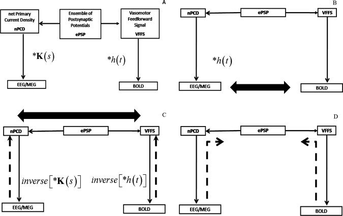
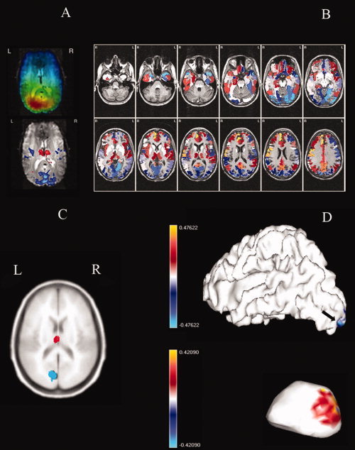
This article reviews progress and challenges in model driven EEG/fMRI fusion with a focus on brain oscillations. Fusion is the combination of both imaging modalities based on a cascade of forward models from ensemble of post-synaptic potentials (ePSP) to net primary current densities (nPCD) to EEG; and from ePSP to vasomotor feed forward signal (VFFSS) to BOLD. In absence of a model, data driven fusion creates maps of correlations between EEG and BOLD or between estimates of nPCD and VFFS. A consistent finding has been that of positive correlations between EEG alpha power and BOLD in both frontal cortices and thalamus and of negative ones for the occipital region. For model driven fusion we formulate a neural mass EEG/fMRI model coupled to a metabolic hemodynamic model. For exploratory simulations we show that the Local Linearization (LL) method for integrating stochastic differential equations is appropriate for highly nonlinear dynamics. It has been successfully applied to small and medium sized networks, reproducing the described EEG/BOLD correlations. A new LL-algebraic method allows simulations with hundreds of thousands of neural populations, with connectivities and conduction delays estimated from diffusion weighted MRI. For parameter and state estimation, Kalman filtering combined with the LL method estimates the innovations or prediction errors. From these the likelihood of models given data are obtained. The LL-innovation estimation method has been already applied to small and medium scale models. With improved Bayesian computations the practical estimation of very large scale EEG/fMRI models shall soon be possible.
2008 Wiley-Liss, Inc.
Figures
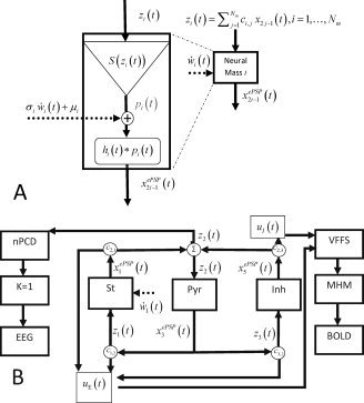
 (dashed arrow). The neural mass produces as an output the ePSPs x
which are also the state variables for this SSM. The ePSPs will feed into other neural masses. Note that z
i(t) is the sum of the ePSPs that are emitted from other connected neural masses, amplified by the synaptic contact coefficients z
i(t) = ∑
c
i,j
x
2j−1(t), where c
i,j indicates connections from population j to i. By convention these synaptic connectivities will be negative for when j is an inhibitory cell. On the left is shown in more detail the sequence of operations which take input to output: 1 − z
i(t) is converted into an average pulse density of action potentials p
i(t) = S(z
i(t)) by a static nonlinear sigmoid function S(v). 2‐The noise input, with mean μi and standard deviation σi, is added to the pulse density. 3 ‐
(dashed arrow). The neural mass produces as an output the ePSPs x
which are also the state variables for this SSM. The ePSPs will feed into other neural masses. Note that z
i(t) is the sum of the ePSPs that are emitted from other connected neural masses, amplified by the synaptic contact coefficients z
i(t) = ∑
c
i,j
x
2j−1(t), where c
i,j indicates connections from population j to i. By convention these synaptic connectivities will be negative for when j is an inhibitory cell. On the left is shown in more detail the sequence of operations which take input to output: 1 − z
i(t) is converted into an average pulse density of action potentials p
i(t) = S(z
i(t)) by a static nonlinear sigmoid function S(v). 2‐The noise input, with mean μi and standard deviation σi, is added to the pulse density. 3 ‐  is converted into the output x
(t) by linear convolutions with the neural PSP impulse responses h
i(t). The complete neural mass model creates two additional signals (not shown) that will act as the two components of the VFSS signal originating the BOLD signal. These are the sum of all EPSP u
E(t) = ∑
c
i,j
x2j−1(t) and all IPSP u
I(t) = −∑
c
i,j
x2j−1(t). B: Model for a Jansen‐Rit Cortical Module. Here N
m = 3. Pyramidal cell (Pyr), stellate cell (St), and inhibitory interneuron (Inh) populations generate ePSPs, denoted respectively by {x
(t), x
(t), x
(t)}. The output of Pyr cells, x
(t), multiplied by c
1,2, c
3,2 drives the St and Inh populations. Pyr receives feedback from St and Inh with coefficients c
2,1, c
2,3 respectively. The only dynamic noise input is to the St Population. On the one hand, the nPCD is the transmembrane PSP of the Pyr population which is equal to the net input PSP z
2(t) generated by the St and Inh populations z
2(t) = c
2,1
x
(t) + c
2,3
x
(t) (EPSP‐IPSP). This is also equal to the EEG with the trivial lead field K = 1. Loosely speaking, this is as though we were actually measuring a Local Field Potential (LFP). On the other hand, The VFFS has two components
is converted into the output x
(t) by linear convolutions with the neural PSP impulse responses h
i(t). The complete neural mass model creates two additional signals (not shown) that will act as the two components of the VFSS signal originating the BOLD signal. These are the sum of all EPSP u
E(t) = ∑
c
i,j
x2j−1(t) and all IPSP u
I(t) = −∑
c
i,j
x2j−1(t). B: Model for a Jansen‐Rit Cortical Module. Here N
m = 3. Pyramidal cell (Pyr), stellate cell (St), and inhibitory interneuron (Inh) populations generate ePSPs, denoted respectively by {x
(t), x
(t), x
(t)}. The output of Pyr cells, x
(t), multiplied by c
1,2, c
3,2 drives the St and Inh populations. Pyr receives feedback from St and Inh with coefficients c
2,1, c
2,3 respectively. The only dynamic noise input is to the St Population. On the one hand, the nPCD is the transmembrane PSP of the Pyr population which is equal to the net input PSP z
2(t) generated by the St and Inh populations z
2(t) = c
2,1
x
(t) + c
2,3
x
(t) (EPSP‐IPSP). This is also equal to the EEG with the trivial lead field K = 1. Loosely speaking, this is as though we were actually measuring a Local Field Potential (LFP). On the other hand, The VFFS has two components  , the sum of excitatory PSP and u
I(t) = c
2,3
x
(t) the inhibitory PSP. The VFSS components are fed into the Metabolic Hemodynamic Model (MHM) which we shall not detail here (see Appendix C) a system of ODE which depends on additional state variables x
7(t),…,x
14(t). The observed BOLD is generated by the Balloon model then is transformed to BOLD by the equation y
2(t) = g
BOLD (x
13(t),x
14(t)).
, the sum of excitatory PSP and u
I(t) = c
2,3
x
(t) the inhibitory PSP. The VFSS components are fed into the Metabolic Hemodynamic Model (MHM) which we shall not detail here (see Appendix C) a system of ODE which depends on additional state variables x
7(t),…,x
14(t). The observed BOLD is generated by the Balloon model then is transformed to BOLD by the equation y
2(t) = g
BOLD (x
13(t),x
14(t)).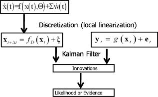
References
-
- Archambeau C,Opper M,Shen Y,Cornford D,Shawe‐Taylor J ( 2007a): Variational inference for diffusion processes In Platt C.,Koller D.,Singer Y.,Roweis S. editors, Neural Information Processing Systems (NIPS) 20, 2008. The MIT Press; Cambridge. Massachusetts: pp. 17–24.
-
- Archambeau C,Cornford D,Opper M,Shawne‐Talyor J. ( 2007b): Gaussian process approximations of stochastic differential equations. JMLR: Workshop and Conference Proceedings. pp. 1–16.
-
- Attwell DF,Iadecola C ( 2002): The neural basis of functional brain imaging signals. Trends Neurosci 25: 621–625. - PubMed
-
- Babajani A,Soltanian‐Zadeh H ( 2006): Integrated MEG/EEG and fMRI model based on neural masses. IEEE Trans Biomed Eng 53: 1794–1801. - PubMed
-
- Babajani A,Nekooei MH,Soltanian‐Zadeh H ( 2005): Integrated MEG and fMRI model: Synthesis and analysis. Brain Topogr 18: 101–113. - PubMed
Publication types
MeSH terms
LinkOut - more resources
Full Text Sources
Medical
