Sensory responses during sleep in primate primary and secondary auditory cortex

Abstract

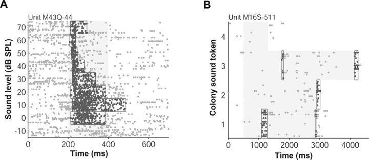
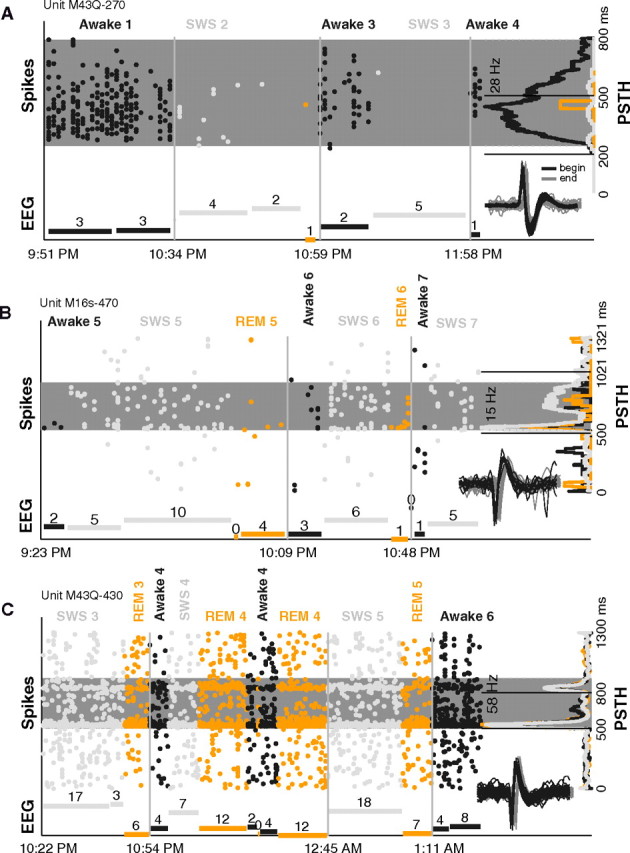
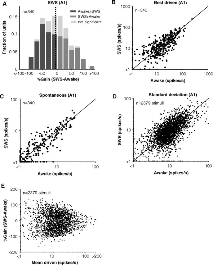
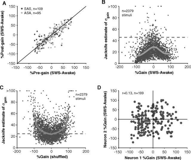
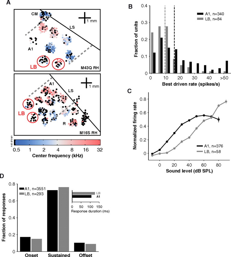
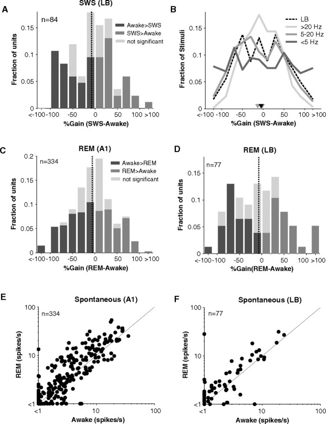
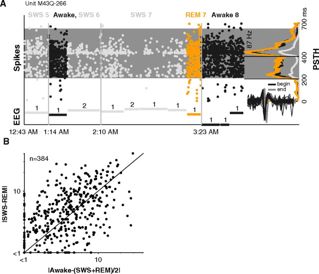
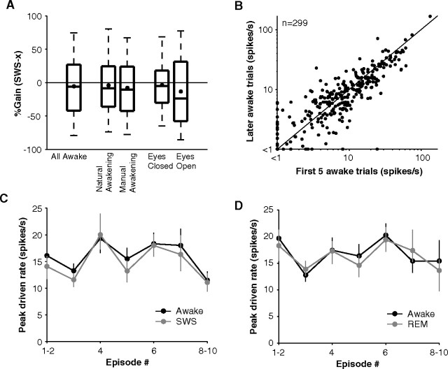
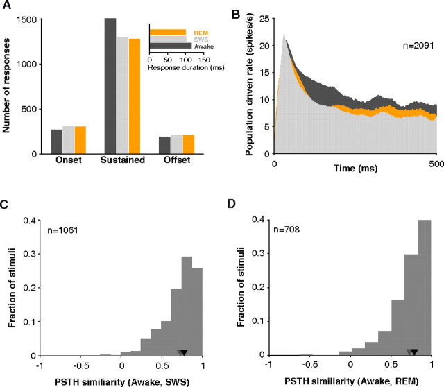
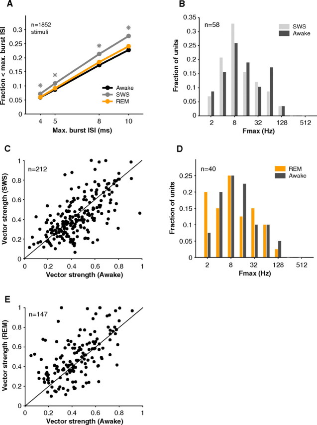
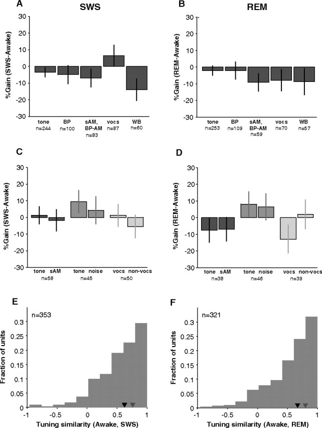
Most sensory stimuli do not reach conscious perception during sleep. It has been thought that the thalamus prevents the relay of sensory information to cortex during sleep, but the consequences for cortical responses to sensory signals in this physiological state remain unclear. We recorded from two auditory cortical areas downstream of the thalamus in naturally sleeping marmoset monkeys. Single neurons in primary auditory cortex either increased or decreased their responses during sleep compared with wakefulness. In lateral belt, a secondary auditory cortical area, the response modulation was also bidirectional and showed no clear systematic depressive effect of sleep. When averaged across neurons, sound-evoked activity in these two auditory cortical areas was surprisingly well preserved during sleep. Neural responses to acoustic stimulation were present during both slow-wave and rapid-eye movement sleep, were repeatedly observed over multiple sleep cycles, and demonstrated similar discharge patterns to the responses recorded during wakefulness in the same neuron. Our results suggest that the thalamus is not as effective a gate for the flow of sensory information as previously thought. At the cortical stage, a novel pattern of activation/deactivation appears across neurons. Because the neural signal reaches as far as secondary auditory cortex, this leaves open the possibility of altered sensory processing of auditory information during sleep.

Figure 1.

Example event windows detected by our algorithm. A, In this example, detected windows (outlines around highlighted spikes) captured the changing duration of the driven response with sound level. B, Windows bracketed the sparse periods of driven firing during long, dynamic sounds recorded in the marmoset colony.

Figure 2.

Example units modulated during sleep. A, Spiking activity and EEG measured during different time points while the animal slept (data were not collected continuously). This unit's response to a sAM tone (carrier frequency = 8.3 kHz, modulation frequency = 256 Hz, sound level = 30 dB SPL) consistently went down when the unit was tested in sleep (gain = −96% in SWS) (dark gray, awake; light gray, SWS; and orange, REM). The spike raster (oriented vertically, each column represents a single trial) shows a clear loss of spiking on entry into SWS in episode 2, a recovery of response on returning to awake in episode 3, and a loss of response again in SWS of episode 4. Far right, The PSTH averages the activity across all trials for each state and is plotted on its side. The clear response in awake is absent in SWS and REM. Gray shaded strip is the analysis window determined by our windowing algorithm. Dashed lines demarcate stimulus playing. Bottom, The normalized EEG amplitude (minimum subtracted) for each epoch tested is shown (times each episode began are marked on abscissa; breaks between EEG bars within an episode denote noncontinuous measurements; and numbers above each bar denote duration of measurement in minutes). When driven spiking is high in awake periods, EEG amplitude is low. In SWS periods, high EEG amplitude accompanies diminished firing. Inset, first 50 (black) and last 50 (gray) spike waveforms collected of the unit during the 2.5-h-long session. Horizontal offset is for display purposes only. B, Same format as A. This unit's response to a marmoset vocalization sound (type = tsik, sound level = 80 dB SPL) went up in SWS (gain = 86% in SWS) but not in REM. Firing rate increased when EEG amplitude (SWS) increased. Session spanned 2 h. C, Same format as A. Unit's response to a tone (frequency = 8.7 kHz, sound level = 60 dB) was similar in awake, SWS, and REM (gain = −11% in SWS). Regardless of multiple large changes in EEG amplitude and behavioral state over the 3-h-long session, the unit remained consistently well driven by the stimulus, and the PSTH retained its distinct onset and offset pattern in all three states.

Figure 3.

Stimulus-driven and spontaneous activity in A1 during awake and SWS. A, Histogram of %Gain (SWS-awake) for neurons recorded in A1 (n = 340). Negative gains are units whose responses went down in SWS. Positive gains represent units whose responses went up in SWS. Lightly shaded portions of bars represent responses that did not significantly differ between awake and SWS (<3× SEM difference). Mean gain = −5% (vertical dotted line). B, Scatter plot of stimulus-evoked firing rates in awake and SWS for the best stimulus of a unit. Maximum driven rates did not significantly differ (p = 0.3, Wilcoxon rank sum, n = 340). C, Scatter plot of unit spontaneous firing rates in awake and SWS. Spontaneous rates did not significantly differ (p = 0.80, Wilcoxon rank sum, n = 340). D, Scatter plot of the SD of firing rates in awake and SWS. SD of driven responses did not significantly differ (p = 0.90, Wilcoxon rank sum, n = 2379). E, %Gain as a function of driven rate for all stimuli tested in A1. No trend is present with driven rate (r² = 2.2*10⁻⁵, p = 0.82, n = 2379).

Figure 4.

Reliability and precision of measured gains in SWS. A, In some units, a recovery control was performed. Modulation of firing was retested in a later sleep cycle. Order of testing was either awake-SWS-awake (ASA) or SWS-awake-SWS (SAS). There was a high correlation between pregains and postgains suggesting similar modulation of a neuron in two separate sleep cycles (r² = 0.71, p = 2.9*10⁻⁵⁶, n = 203). B, SDs of gains, estimated using the jackknife technique, were used to approximate noise arising from inherent variability in neural firing rates and behavioral state. Noise levels at each gain (solid gray line represents mean) were a decreasing function of the absolute value of gain. Especially for high gains, noise was low. The mean 46% change in firing rate observed during SWS (dashed gray line) was generally above noise levels (mean = 21%). C, If individual trials are randomly assigned to awake or SWS, the magnitude of gain becomes positively correlated with noise in the measurement. High gains are simply the result of high variability in firing rates. This was not the trend in B, suggesting a systematic effect of sleep beyond measurement noise. D, SWS modulation of neurons recorded within 200 μm of each other. Gains of neighboring neurons were not correlated (r² = 0.02, p = 0.06, n = 199). Often neurons were modulated in opposite directions (top left and lower right quadrant of plot) such that the response of one neuron would increase on entry to SWS (positive gain) whereas the response of a second, nearby neuron would decrease (negative gain).

Figure 5.

Recording maps and properties of lateral belt. A, LB recordings were obtained in the right hemispheres of 2 animals in addition to A1 recordings. The tonotopic progression in A1 can be seen in the maps of both animals. In animal M43q (top), A1 was bounded caudally by CM (caudomedial field). In animal M16 s (bottom), A1 was bounded rostrally by R (rostral field). In both cases a clear frequency reversal is seen at the borders (dashed lines). Colored dots indicate neurons whose center frequencies were determined. The dots are slightly dispersed for display purposes. Black dots represent track locations in which center frequencies were not determined because neurons were unresponsive to tones or narrowband noise. LB recordings (red circles) were made far from the lateral sulcus (LS, diagonal black line). These regions had weak overall responses and poor tonotopic gradients as evidenced by the prevalence of black dots. B, Units in LB were not driven as strongly as units in A1 (median best response LB = 9.5 vs A1 = 15.9, p = 9.6*10⁻⁸, Wilcoxon rank sum, n_LB = 84, n_A1 = 340). Vertical dashed lines represent medians. C, Population rate levels in A1 (n = 376) and LB (n = 58). Curves from either awake or SWS were normalized by peak response and then summed. Activity in LB was more monotonic (grows with sound level) than in A1. Error bars represent ±0.5× SEM. D, Windows detected by our algorithm were classified as onset, offset, or sustained (see Materials and Methods). In both A1 and LB, sustained windows were the dominant form of response under the awake condition. Responses lasted slightly longer in LB (mean = 126 ms) than in A1 (mean = 106 ms) (inset).

Figure 6.

Stimulus-driven and spontaneous activity in LB during sleep. A, Histogram of %Gain (SWS-awake) for cells recorded in LB (n = 84). Mean gain = −8% (vertical dotted line). Same format as Figure 3A. B, Control for effects of firing rate in comparing A1 and LB. Dividing the A1 data into low (0–5 Hz), middle (5–20 Hz), and high (>20 Hz) firing rates yielded three gain distributions of near-identical medians (−3%, −13%, and −4% respectively) (inverted triangles) but increasing variance (SD = 72%, 54%, 43%). The gain distribution was tightest for high firing rates. The distribution for LB (black, dashed line) fell on the A1 distribution for intermediate firing rates (5–20 Hz) consistent with LB rates averaging 8 Hz. C, D, Gain histograms in REM for A1 (C) and LB (D). Mean gain = −5% (A1) and −7% (LB) (vertical dashed lines). E, F, Scatter plots of spontaneous firing rates in A1 (E) and LB (F). Although a trend toward higher REM spontaneous rates appears to be present, spontaneous rates were not significantly different from those in awake whether in A1 or LB (p_A1 = 0.23, p_LB = 0.31, Wilcoxon rank sum, n_A1 = 334, n_LB = 77).

Figure 7.

Lack of similarity between SWS and REM responses. A, Same format as Figure 2. Example unit that responded strongly in REM (gain = +8%) but not in SWS (gain = −69%) to a pure tone (frequency = 12.7 kHz, sound level = 60 dB SPL). The unit's response in REM was similar to awake, but in three different occurrences of SWS, the SWS response was much weaker than the REM response. Windowing algorithm captured the significant 250 ms portion of the response which extended well beyond stimulus offset (gray shaded region). Unit was well isolated at beginning and end of the ∼4-h-long recording (see inset spike waveforms). B, Difference between SWS and REM firing rates plotted against the difference from awake rate. Firing rates in SWS and REM were no more similar to each other (median difference = 4.6 spikes/s) than they were to awake (median difference = 3.8 spikes/s) (p = 0.008, Wilcoxon rank sum, n = 384).

Figure 8.

Arousal controls and stability of responses throughout the night. A, %Gain (SWS-awake) recomputed under different arousal conditions. Far left box plot represents SWS gain distribution when all awake conditions were used for comparison (n = 424). Middle box plots compare gains for natural (animal awakens and falls back asleep on its own) versus manual (experimenter induced) awakenings in units tested in both conditions (n = 139). Right bars compare gain for eye-open versus eye-closed trials in units in which at least four trials were collected in both conditions (n = 84). Box plots are divided into quartiles, and whiskers represent 5th to 95th percentile. B, Comparison of awake firing rates for the first five trials after awakening and the remaining trials the animal was awake before falling back asleep. It might be expected that firing would be strongest immediately when the animal awakened, but firing rates did not significantly differ from those before the animal became drowsy again and fell back asleep (p = 0.64, Wilcoxon rank sum, n = 299). C, Trend in population activity over the course of the night (error bars represent ±SEM). Recordings were performed throughout the night starting from when the animal first fell asleep until the early morning. No clear trend in either awake or SWS responses was present, and the two curves follow each other, representing the idiosyncrasies of the population of neurons sampled during each episode. D, Same format as in C except for REM responses in comparison to awake responses.

Figure 9.

Response patterns observed in sleep. A, The number of sustained responses dropped slightly in sleep (SWS or REM) as reflected in the shorter average duration of detected responses (inset). B, Population response profiles for all stimuli tested in awake, SWS, and REM. Population PSTH was obtained by averaging, without normalizing, all responses during their respective driven windows. Responses were long-lasting in all three states. C, The distribution of similarity values (Pearson's product–moment correlation coefficient) between PSTH profiles in awake and SWS. Response patterns were highly correlated (median = 0.78, n = 1061; black inverted triangle) especially when compared with correlation attainable using odd and even trials from the same state (gray triangle). D, The distribution of similarity values between PSTH profiles in awake and REM. Response patterns were highly correlated (median = 0.79, n = 708; black inverted triangle).

Figure 10.

Bursting and stimulus synchronization in sleep. A, Neurons tended to be burstier (fraction of interspike intervals < maximum ISI) in SWS. Awake and REM spike trains had similar burst fractions. Asterisks represent significance at the p < 0.001 level in comparison of SWS to awake and REM (Wilcoxon rank sum, n = 1852 stimuli). B, Comparison of upper limit of stimulus synchronization (F_max) in awake (dark gray) and SWS (light gray). In general, neurons were able to follow up to similar repetition frequencies in both states (mean F_max awake = 14.0, SWS = 11.6 Hz, p = 0.37, Wilcoxon rank sum, n = 58). C, Vector strengths in awake and SWS were comparable (mean VS awake = 0.45, SWS = 0.43, p = 0.11, Wilcoxon rank sum, n = 212). D, F_max distributions were similar in awake and REM (mean awake = 12.7, REM = 10.2 Hz, p = 0.46, Wilcoxon rank sum, n = 40). E, Vector strength in REM was similar to that in awake (mean VS awake = 0.44, REM = 0.49, p = 0.07, Wilcoxon rank sum, n = 147).

Figure 11.

Sleep modulation of all neurons tested across stimulus classes. A, We used five main stimulus types to probe neural responses [tones, bandpass noise (BP), sinusoidal amplitude modulated tones (sAM) or noise (BP-sAM), vocalizations (vocs), and wideband noise (WB)]. In general, gains were somewhat negative but not different from 0% (p > 0.05, bootstrap; n = 10,000 simulations in which awake and SWS firing rates were randomly exchanged) except for wideband noise (p = 0.05, bootstrap). B, Gains in REM for the five main stimulus types were not different from 0% (p > 0.05, bootstrap). C, In many cases, more than one stimulus type was tested on a neuron, and direct comparisons could be made within a neuron. No difference was found in SWS gain for unmodulated versus modulated tones (p = 0.64, n = 58), for tones versus narrowband stimuli (p = 0.47, n = 45), and for vocalizations versus nonvocalization stimuli (p = 0.34, n = 50) (Wilcoxon rank sum) (similarly shaded pairs of bars represent data from two different stimulus types collected in the same neuron). Gain remained near 0% in all cases. D, Within-unit comparisons of the effects of REM did not reveal any difference in sleep gains for modulated (p = 0.95, n = 38), larger-bandwidth (p = 0.98, n = 46), or semantically meaningful (p = 0.22, n = 39) (Wilcoxon rank sum) stimuli. E, The similarity between awake and SWS firing rate profiles (see Materials and Methods) across all stimuli was relatively high (median ρ = 0.63, n = 353; black inverted triangle) but not as high as within-state similarity (median = 0.76, n = 704; gray inverted triangle). F, Awake and REM firing rate profiles across all stimuli also tended to be highly correlated (median ρ = 0.67, n = 321; black inverted triangle).

References

1. BarthóP, Hirase H, Monconduit L, Zugaro M, Harris KD, Buzsáki G (2004) Characterization of neocortical principal cells and interneurons by network interactions and extracellular features. J Neurophysiol 92:600–608. - PubMed
1. BastujiH, Perrin F, Garcia-Larrea L (2002) Semantic analysis of auditory input during sleep: studies with event related potentials. Int J Psychophysiol 46:243–255. - PubMed
1. BehHC, Barratt PE (1965) Discrimination and conditioning during sleep as indicated by the electroencephalogram. Science 147:1470–1471. - PubMed
1. BensonDA, Hienz RD (1978) Single-unit activity in the auditory cortex of monkeys selectively attending left vs. right ear stimuli. Brain Res 159:307–320. - PubMed
1. BonnetMH (1982) Performance during sleep. In: Biological rhythms, sleep and performance (Webb WB, ed), pp 205–237. Chichester, UK: Wiley.
Publication types
LinkOut - more resources