. 2009 Jan 20;7(1):e15.
doi: 10.1371/journal.pbio.1000015.

Cell lineages and the logic of proliferative control

Affiliations

Cell lineages and the logic of proliferative control

Arthur D Lander et al. PLoS Biol. .

Abstract

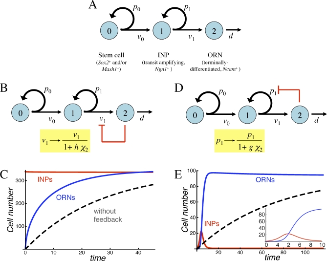
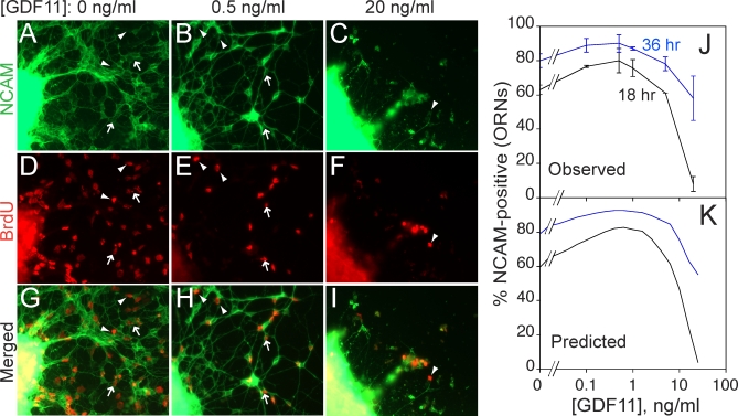
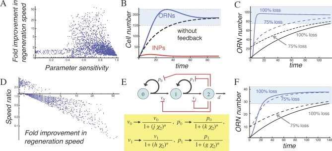
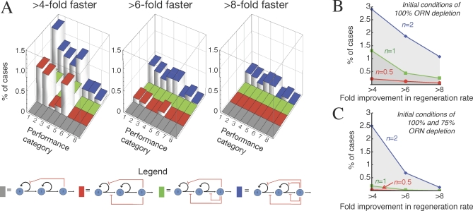
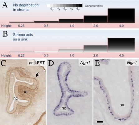
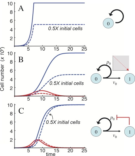
It is widely accepted that the growth and regeneration of tissues and organs is tightly controlled. Although experimental studies are beginning to reveal molecular mechanisms underlying such control, there is still very little known about the control strategies themselves. Here, we consider how secreted negative feedback factors ("chalones") may be used to control the output of multistage cell lineages, as exemplified by the actions of GDF11 and activin in a self-renewing neural tissue, the mammalian olfactory epithelium (OE). We begin by specifying performance objectives-what, precisely, is being controlled, and to what degree-and go on to calculate how well different types of feedback configurations, feedback sensitivities, and tissue architectures achieve control. Ultimately, we show that many features of the OE-the number of feedback loops, the cellular processes targeted by feedback, even the location of progenitor cells within the tissue-fit with expectations for the best possible control. In so doing, we also show that certain distinctions that are commonly drawn among cells and molecules-such as whether a cell is a stem cell or transit-amplifying cell, or whether a molecule is a growth inhibitor or stimulator-may be the consequences of control, and not a reflection of intrinsic differences in cellular or molecular character.


Conflict of interest statement

Competing interests. The authors have declared that no competing interests exist.

Figures

Figure 1
Figure 1. Biological Pathways That Are Potential Targets of Control
Like metabolic, signaling, and gene expression pathways, cell lineages may be viewed as input–output pathways in which information or material flows through a series of defined elements (A–D) at rates controlled by measurable parameters (e.g., enzyme levels E 1, E 2, synthesis rates v 1, v 2, etc.). Unlike these other pathways, cell lineages are characterized by a potential for exponential expansion at most or all stages (parameters p 0, p 1, etc.). The impact of this difference on the strategies that may be used for tissue growth control has been little studied.
Figure 2
Figure 2. Lineage Behavior in the Absence of Control
(A) Cartoon of an unbranched lineage that begins with a stem cell (type 0), progresses through an arbitrary number of transit-amplifying stages (types 1 to n − 1) and ends with a postmitotic terminal-stage cell (type n). Parameters v i and p i are the rate constants of cell cycle progression and the replication probabilities, respectively, for each stage. Turnover of the terminal-stage cell is represented with a cell-death rate constant, d. (B) Representation of the cell lineage shown in (A), as a system of ordinary differential equations. In these equations, χi(t) stands for the number (or concentration) of cells of type i at time t, with each equation expressing the rate of expansion (or contraction) of each cell type. For all cell types except the first and last, this rate is the sum of two terms: production by cells of the previous lineage stage, and net production (or loss) due to replication (or differentiation) of cells at the same lineage stage. For the first cell type, there is no production from a prior stage, and for the last cell type, loss due to cell death is included. (C) Steady state solution for the output (number of terminal-stage cells) of the general system of equations given in (B). Notice that this output is linearly, or more than linearly, sensitive to every system parameter, with the exception of the v i for i > 0, which do not appear in the solution.
Figure 3
Figure 3. Strategies for Feedback Regulation of Transit-Amplifying Cells
(A) The neuronal lineage of the OE, in which terminally differentiated ORNs are produced by committed transit-amplifying cells (INPs). (B) Negative feedback regulation of the INP cell cycle length (shown diagrammatically in red) can be modeled by making v 1 a function of ORN numbers (χ 2). (C) Simulated return to steady state of the system in (B) after removal of all ORNs. The parameters chosen provide the greatest improvement in regeneration speed (over what would occur in the absence of feedback; dashed line), consistent with progenitor cells comprising no more than 50% of the tissue mass (note that INP numbers [red curve] are virtually the same as those of ORNs [blue curve] at steady state). Cell numbers are expressed relative to the starting number of stem cells. (D) Negative feedback regulation of the INP replication probability (shown diagrammatically in red) can be modeled by making p 1 a function of ORN levels (χ 2). (E) Simulated return to steady state of the system in (D) after removal of ORNs. An inset shows the response at early times in greater detail. Note that progenitor load is now quite low, and regeneration is characterized by a burst of INP proliferation (red curve), followed by a wave of ORN production (blue curve). In (C and E), time is expressed in units of ln2/v 1. Parameter values for (C) are p 1 = 0.495, d/v 1 = 0.0372, v 0/v 1 = 0.128, and h = 0.0734, and for (E) are p 1 = 0.942, d/v 1 = 0.0138, v 0/v 1 = 0.506, and g = 0.0449.
Figure 4
Figure 4. Experimental Demonstration That GDF11 Regulates p 1 and v 1
OE explants were cultured in various doses of GDF11. At 12 h, BrdU was added for 2 h and then washed out. Explants were fixed at various times after BrdU addition and immunostained for BrdU and NCAM expression. (A–I) Cultures grown in GDF11 concentrations of 0 (A, D, and G), 0.5 (B, E, and H), and 10 (C, F, and I) ng/ml, fixed 18 h after BrdU addition (previous studies have shown that 18 h is sufficient time for INP progeny that become ORNs to express NCAM [39]). NCAM immunofluorescence (green) is shown in (A–C); BrdU immunofluorescence (red) in (D–F); merged images in (G–I). Arrowheads point to examples of BrdU+/NCAM cells; arrows point to examples of BrdU+/NCAM+ cells. (J) Percentage of BrdU+ cells migrating out of OE explants that had differentiated (acquired NCAM immunoreactivity) by 18 h (black line) or 36 h (blue line), as a function of GDF11 dose. Low doses of GDF11 increase the proportion of INP progeny that differentiate (i.e., p 1 decreases). At high dose, the effect reverses, with the NCAM+ fraction falling to near zero at 18 h, but recovering at 36 h. These data are consistent with a slowing of the cell cycle (v 1) such that 18 h is not long enough to produce NCAM+ offspring (but 36 h is). This interpretation is consistent with a previous demonstration that high doses of GDF11 reversibly arrest the INP cell cycle [34]. (K) Simulation of the experiment in (J) by a model in which GDF11 affects both p 1 and v 1. Parameters used in the model are consistent with measured proportions of ORNs, INPs, and Mash1 +/Sox2 + cells, as well as experimental data on the effects of GDF11 on BrdU pulse-labeling by INPs [34,39,40].
Figure 5
Figure 5. Performance Tradeoffs Associated with Feedback Strategies
(A) Simulations of the model in Figure 3D were carried out for 20,000 randomly chosen sets of parameters (Protocols S1–S3, section 8). To simulate regeneration following a loss of terminal-stage cells, numbers of ORNs were set to zero, whereas numbers of stem cells and transit-amplifying cells (INPs) were set to their steady state values. For each parameter set, the time it took for ORN numbers to return to and remain within 20% of their steady state values was taken as an objective measure of regeneration time, and cases with very long regeneration times (>29 transit-amplifying cell cycle lengths) are not shown (see Protocols S1–S3). Next, the time that would have been required to generate the same number of ORNs, from the same initial conditions but in the absence of feedback, was calculated. Finally, the ratio of the two regeneration times (with and without feedback) was considered to be the fold improvement in regeneration speed due to feedback. For each parameter set, this was plotted against the sensitivity of the steady state solution to variation in either the initial number of stem cells, the stem cell cycle time, or the normal lifetime of ORNs (all three sensitivities are equal). The data show that only those parameter sets that do not support a robust ORN steady state (abscissa values >0.4) show substantial improvement in regeneration speed (ordinate values >2). (B) Simulated regeneration for the set of parameters in (A) that showed the greatest improvement in regeneration consistent with sensitivity to parameters remaining below 0.4 (this corresponds to a 32% change in steady state values for a 2-fold change in parameters). As in Figure 3, the blue curve denotes ORN numbers, the red curve shows INPs, and the dashed line shows the time course over which regeneration would proceed in the absence of feedback. The light-blue zone denotes the range of cell numbers within 20% of the steady state value for ORNs. (C) Simulated regeneration for the parameters used in Figure 3C, but starting from two different initial conditions. The solid blue curve shows the dynamics of ORN recovery after complete removal of existing ORNs; the solid gray curve illustrates the predicted rate of recovery in the absence of feedback. The dashed blue and gray curves present corresponding simulations where ORN numbers were initially depleted only 75%, rather than completely. Under these conditions, nearly all improvement in regeneration is lost. (D) To quantify the effect of initial conditions on regeneration speed, a ratio was defined (“speed ratio”) that indicates how much faster (or slower) regeneration from 75% ORN depletion is than regeneration from 100% depletion. In the absence of feedback, this ratio should have a value of approximately 1.22 (regeneration from partial depletion should take slightly less time than regeneration from total depletion). This ratio was calculated for each of the random cases shown in (A), and the results were plotted against the fold improvement in regeneration speed (from [A]). The abscissa is drawn at an ordinate value of 1.22. The plot shows that the more one gains in regeneration speed from 100% depletion, the more one sacrifices in regeneration speed from 75% depletion. (E) Negative feedback effects of activin and GDF11 (shown diagrammatically in red) can be modeled by multiplying the replication probabilities and cell division rates of stem cells and INPs, respectively, by decreasing functions of ORN numbers (χ2). In this case, Hill functions are used, with parameters g, h, j, and k representing the feedback gains, and n the Hill coefficient. (F) Example of a case with both activin and GDF11 feedback. Notice that now, regeneration from initial conditions of 75% ORN depletion is nearly as fast as regeneration from 100% ORN depletion (compare with [C]). Parameters for this case are: p 0 = 0.507, p 1 = 0.546, d/v 1 = 0.0116, v 0/v 1= 0.965, g = 1.258, h = 1.03, j = 0.0394, and k = 1.683 (and the ordinate axis has been scaled for easier comparison with [C]). In (B), (C), and (F), time is expressed in units of ln2/v 1.
Figure 6
Figure 6. Effects of Feedback Configuration on Regeneration from Diverse Perturbations
(A) Four different feedback architectures (shown diagrammatically beneath the word “Legend”) were modeled and investigated for their ability to support rapid regeneration from multiple starting conditions. For each model, 20,000 random parameter sets were explored (see Protocols S1–S3, section 8) using simulations that started from initial conditions corresponding to four different perturbations of the steady state. For all 640,000 solutions, the fold improvement in ORN regeneration speed was calculated as in Figure 5. The bar graphs depict the fractions of random parameter sets for each model that produced at least a given amount of improvement in regeneration speed for one or more sets of initial conditions. The four different feedback architectures are designated by different colored bars (see diagrams under “Legend”): feedback on p 0 (grey); p 0 and v 0 (red); p 0, v 0, and v 1 (green); and p 0, v 0, p 1, and v 1 (blue). The heights of bars give the fraction of parameter sets that produced at least the indicated amount—4-fold (left graph), 6-fold (middle graph), or 8-fold (right graph)—of improvement in regeneration speed. The “Performance categories” refer to different combinations of initial conditions: Cases included in performance category 1 are those that met the desired level of improvement in the speed of regeneration following a complete loss of terminal-stage cells. In category 2, the perturbation was a complete loss of both terminal-stage and transit-amplifying cells. In category 3, it was a 75% loss of terminal-stage cells. In category 4, the perturbation was a complete loss of terminal-stage and transit-amplifying cells and a 50% loss of stem cells. Category 5 cases are those parameter sets that met the criteria for initial conditions of both categories 1 and 2. Category 6 refers to those that did so for both categories 1 and 3. Category 7 refers to those that did so for both categories 1 and 4. Category 8 refers to cases in which the parameter sets met the indicated criterion for all four initial conditions. The data show that rapid regeneration from a variety of initial conditions is facilitated by feedback on the p-parameters of at least two progenitor cell stages. (B and C). For the system with feedback on p 0, v 0, p 1, and v 1 (i.e., the system depicted with blue bars in [A]), the graphs show the percentages of random parameter sets that meet the regeneration-rate criteria on the abscissa (4-fold, 6-fold, or 8-fold improvement in regeneration speed), as a function of the Hill coefficient, n, used in the expressions for the feedback functions. The results in (B) were obtained by only considering simulations that started from a 100% loss of terminal-stage cells. Cases presented in (C) are those that also met the same regeneration-rate criteria for simulations starting from a 75% loss of terminal-stage cells. The results show that larger n substantially increases the fraction of cases with rapid regeneration. This effect is especially prominent when the performance criteria call for fast regeneration from more than one set of initial conditions (C).
Figure 7
Figure 7. Effects of Geometry and Degradation on Levels of Secreted Molecules within Epithelia
(A and B) Polypeptides secreted into the intercellular space of an epithelium are removed by two processes: diffusion into underlying connective tissue (stroma) and degradation within the epithelium. Given a molecule's rate of production, its diffusivity, its rate of uptake and degradation, and the geometry of the epithelium, one may calculate its concentration, at steady state, at every location within the epithelium. Here, such calculations are shown graphically, for epithelia of different thicknesses (in each picture, the epithelium is oriented with the apical surface at the top). Epithelial thickness (“height”) is scaled according to the decay length of the molecule of interest. The shading in each picture depicts the concentration of the secreted molecule, with black representing the limiting concentration that would be achieved in an epithelium of infinite thickness. In (A), the degradation capacity of the stroma is set at a relatively low value, one-tenth of that in the epithelium. In this case, intraepithelial concentrations of secreted molecules plateau while the epithelium is very thin. In (B), the degradation capacity of the stroma is ten times of that in the epithelium, so that few molecules that enter the stroma escape undegraded. Now, there is a large (and more physiological) range of epithelial thickness over which the concentrations of secreted molecules change appreciably with tissue size. This is particularly true near the basal surface of the epithelium (see also Figures S27 and S28 in Protocols S1–S3). (C) Follistatin (FST), a molecule that binds GDF11 and activin essentially irreversibly, is present at high levels in the basal lamina (arrow) and stroma (asterisk) beneath the embryonic day 13 OE. Association of FST with basal laminae is consistent with its affinity for extracellular matrix components [102]. Scale bar represents 100 μm. (D and E) INPs (visualized with Ngn1 in situ hybridization) become progressively localized to the basal surface of the OE over the course of development. (D) = embryonic day 12.5; (E) = embryonic day 18.5. nc = nasal cavity. Scale bar in (E) represents 100 μm.
Figure 8
Figure 8. Behaviors of Final-State Systems
Three different ways are shown by which an initial pool of 105 progenitors (solid curves) or 5 × 10⁴ progenitors (dashed curves) can generate 108 terminally differentiated cells. Differences among the three mechanisms are illustrated by the diagrams at right. (A) Simple exponential expansion. The progenitor pool expands for just enough time to produce the desired output and then stops. Halving the starting number of progenitors halves the output. (B) Nowakowski-Caviness system: progenitors undergo both replicative and differentiative divisions, according to a replication probability p 0, which starts at p max > 0.5 and declines linearly to p min < 0.5 at time τ. As in (A), halving the initial progenitor cell number halves the output. The output is also highly sensitive to values of p max and τ. (C) System with negative feedback on p 0. Feedback is modeled as previously, using a Hill function (without cooperativity in this example). Halving the starting progenitor pool now produces almost no change in output (there is, however, a one cell cycle lag in reaching the final state). Sensitivity to p 0 is also reduced. In each panel, time is expressed in units of ln2/v 1. Parameter values were, in (A), time of cessation of cell division = 6.91/v 0; in (B), p max = 1, p min = 0, and τ = 19.4; and in (C), p 0 = 0.9, and γ = 3.14 × 10⁸ (where γ is the feedback gain).

Comment in

Similar articles

Cited by

References

    1. Dzierzak E, Speck NA. Of lineage and legacy: the development of mammalian hematopoietic stem cells. Nat Immunol. 2008;9:129–136. - PMC - PubMed
    1. Stern CD, Fraser SE. Tracing the lineage of tracing cell lineages. Nat Cell Biol. 2001;3:E216–218. - PubMed
    1. Fichelson P, Audibert A, Simon F, Gho M. Cell cycle and cell-fate determination in Drosophila neural cell lineages. Trends Genet. 2005;21:413–420. - PubMed
    1. Iwasaki H, Akashi K. Myeloid lineage commitment from the hematopoietic stem cell. Immunity. 2007;26:726–740. - PubMed
    1. Shostak S. (Re)defining stem cells. Bioessays. 2006;28:301–308. - PubMed

Publication types