Variance components linkage analysis with repeated measurements

Abstract

Background: When subjects are measured multiple times, linkage analysis needs to appropriately model these repeated measures. A number of methods have been proposed to model repeated measures in linkage analysis. Here, we focus on assessing the impact of repeated measures on the power and cost of a linkage study.

Methods: We describe three alternative extensions of the variance components approach to accommodate repeated measures in a quantitative trait linkage study. We explicitly relate power and cost through the number of measures for different designs. Based on these models, we derive general formulas for optimal number of repeated measures for a given power or cost and use analytical calculations and simulations to compare power for different numbers of repeated measures across several scenarios. We give rigorous proof for the results under the balanced design.

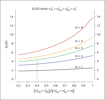
Results: Repeated measures substantially improve power and the proportional increase in LOD score depends mostly on measurement error and total heritability but not much on marker map, the number of alleles per marker or family structure. When measurement error takes up 20% of the trait variability and 4 measures/subject are taken, the proportional increase in LOD score ranges from 38% for traits with heritability of approximately 20% to 63% for traits with heritability of approximately 80%. An R package is provided to determine optimal number of repeated measures for given measurement error and cost. Variance component and regression based implementations of our methods are included in the MERLIN package to facilitate their use in practical studies.

Fig. 1

Expected LOD score for 1000 nuclear families with 4 offspring, where σ²_mg = 0.2, σ²_pg = 0,…, 0.8, σ²_e = 0.8 − σ²_pg and σ²_m = σ²_mg + σ²_pg + σ²_e = 1. m = the number of repeated measures.

Fig. 2

Contour plot for optimal number of repeated measures when the cost ratio ranges from 0 to 50 and σ²_m ranges from 0.11 to 1.5 (10–60% of total trait variance). Trait variance excluding measurement error is fixed to 1 (σ²_mg = 0.2, σ²_pg = 0.4, σ²_e = 0.4). The numbers on the plot indicate the optimal number of repeated measures.

Fig. 3

Average LOD score profile for balanced design simulations (scenario 2). σ²_m = 67 (40% total variance), σ²_pg = 40 (24%). Results based on 500 simulation replications and plotted at every 1 Mb grid point.

Fig. 4

Contour plot of optimal number of repeated measures when the cost ratio ranges from 0 to 30 and σ²_m ranges from 11 to 150 (10–60% total variance). Trait variance excluding measurement error is fixed to 100 (σ²_mg = 20, σ²_pg = 40, σ²_e = 40). This setting is equivalent to the setting in figure 2. Each line separates two regions in which one design is better than the other. For example, to the left of the (blue) dot line, balanced design m = 1 is better than the unbalanced design m = 1.2; on the right side of the line, the unbalanced design m = 1.2 is better than balanced design m = 1. Note that the (blue) dot line is to the right of the (red) dash line, thus balanced designs are superior to unbalanced designs in any situation. For the region to the right of the grey (green) solid line, the optimal design is balanced design m = 4; for the region between the black solid line and the grey (green) solid line, the optimal design is balanced design m = 2; for the region to the left of the black solid line, the optimal design is balanced design m = 1.

Fig. 5

ELOD ratio of full model vs. average model for unbalanced design. Setting is scenario 2. Left 4 pairs of bars are for σ²_m = 11 (10% of total variance). Right 4 pairs of bars are for σ²_m = 150 (60% of total variance). Random design: the number of repeated measures follows an exponential distribution. Extreme design: 20% subjects with extreme first measure have an additional measurement.

References

-
- Boomsma DI, Dolan CV. A comparison of power to detect a QTL in sib-pair data using multivariate phenotypes, mean phenotypes, and factor scores. Behav Genet. 1998;28:329–340. - PubMed
- Levy D, DeStefano AL, Larson MG, O'Donnell CJ, Lifton RP, Gavras H, Cupples LA, Myers RH. Evidence for a gene influencing blood pressure on chromosome 17. Genome scan linkage results for longitudinal blood pressure phenotypes in subjects from the Framingham heart study. Hypertension. 2000;36:477–483. - PubMed
- de Andrade M, Gueguen R, Visvikis S, Sass C, Siest G, Amos CI. Extension of variance components approach to incorporate temporal trends and longitudinal pedigree data analysis. Genet Epidemiol. 2002;22:221–232. - PubMed
Publication types
MeSH terms
Substances
Grants and funding
LinkOut - more resources
Full Text Sources
Other Literature Sources