Three-dimensional linear system analysis for breast tomosynthesis

Abstract

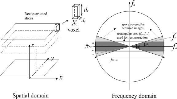
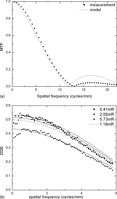
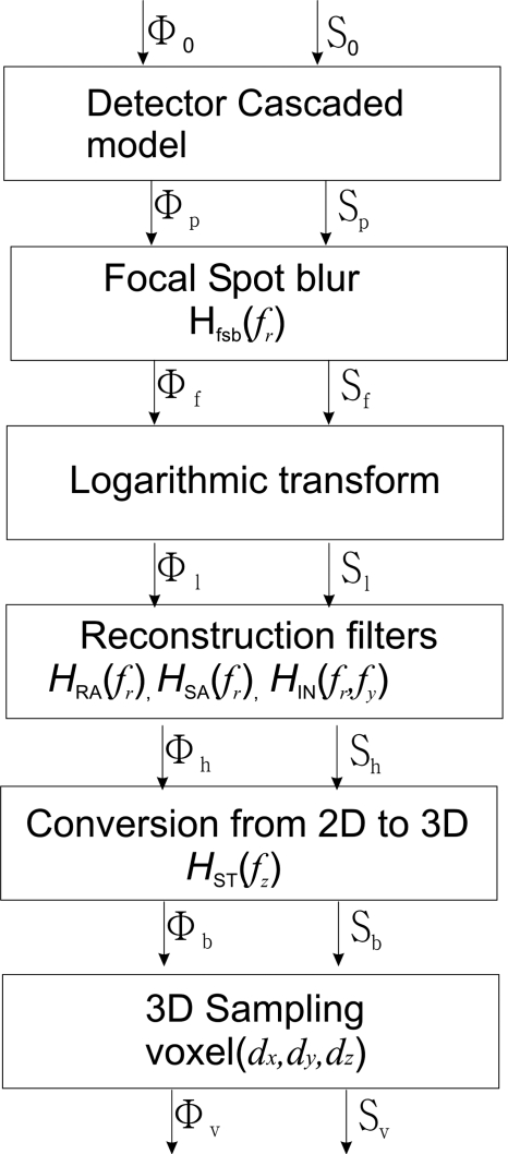
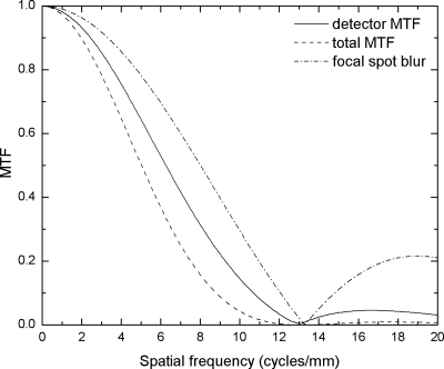
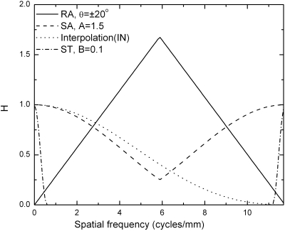
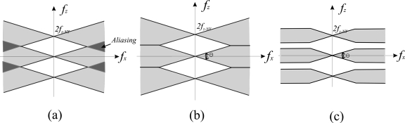
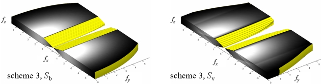
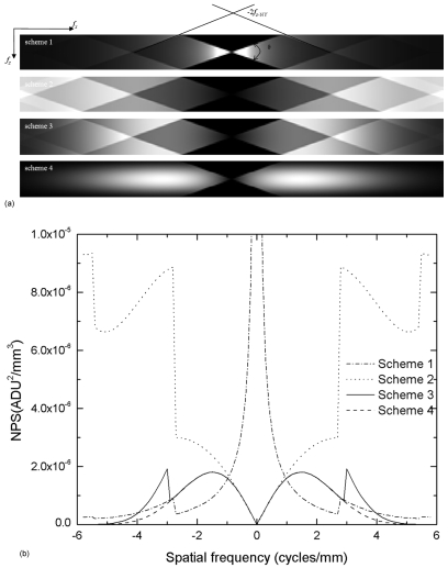
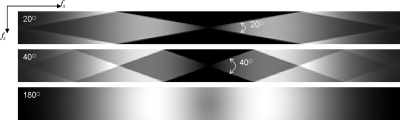
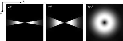
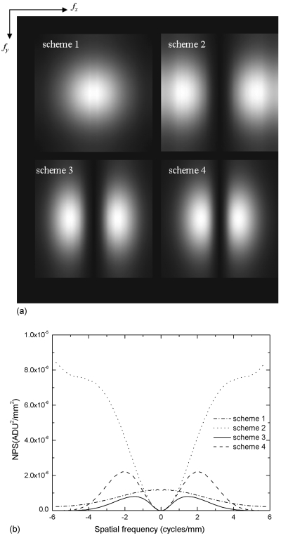
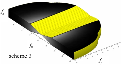
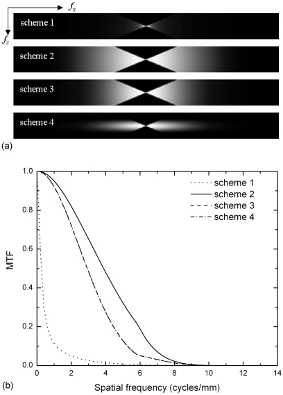
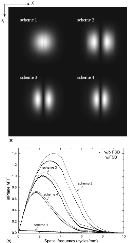
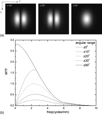
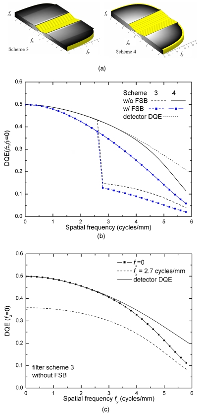
The optimization of digital breast tomosynthesis (DBT) geometry and reconstruction is crucial for the clinical translation of this exciting new imaging technique. In the present work, the authors developed a three-dimensional (3D) cascaded linear system model for DBT to investigate the effects of detector performance, imaging geometry, and image reconstruction algorithm on the reconstructed image quality. The characteristics of a prototype DBT system equipped with an amorphous selenium flat-panel detector and filtered backprojection reconstruction were used as an example in the implementation of the linear system model. The propagation of signal and noise in the frequency domain was divided into six cascaded stages incorporating the detector performance, imaging geometry, and reconstruction filters. The reconstructed tomosynthesis imaging quality was characterized by spatial frequency dependent presampling modulation transfer function (MTF), noise power spectrum (NPS), and detective quantum efficiency (DQE) in 3D. The results showed that both MTF and NPS were affected by the angular range of the tomosynthesis scan and the reconstruction filters. For image planes parallel to the detector (in-plane), MTF at low frequencies was improved with increase in angular range. The shape of the NPS was affected by the reconstruction filters. Noise aliasing in 3D could be introduced by insufficient voxel sampling, especially in the z (slice-thickness) direction where the sampling distance (slice thickness) could be more than ten times that for in-plane images. Aliasing increases the noise at high frequencies, which causes degradation in DQE. Application of a reconstruction filter that limits the frequency components beyond the Nyquist frequency in the z direction, referred to as the slice thickness filter, eliminates noise aliasing and improves 3D DQE. The focal spot blur, which arises from continuous tube travel during tomosynthesis acquisition, could degrade DQE significantly because it introduces correlation in signal only, not NPS.

Figure 1

Diagrams showing the data sampling of the reconstructed images for DBT in the spatial domain (left) and spatial frequency domain (right). The area shaded in light gray with an angular range of θ shows the sampled frequency range as determined by the central slice theorem. The area shaded in darker gray indicates the frequency range below the Nyquist frequencies in both the x (tube travel) and z (slice thickness) directions. As described later in the article, frequency limiting filters, such as the slice thickness filter, can be applied in the FBP process to minimize aliasing in the reconstruction process.

Figure 2

Comparison between measured and modeled detector performance for an a-Se digital detector with 85 μm pixel size used in breast tomosynthesis: (a) MTF and (b) DQE.

Figure 3

Flow chart for signal and noise propagation in the cascaded linear system model.

Figure 4

Modeled presampling MTF curves to show the effect of FSB. The image acquisition parameters are shown in Table 1. The FSB was calculated for a DBT system with a stationary detector.

Figure 5

Reconstruction filters plotted as a function of spatial frequency for full detector resolution, which corresponds to f_NY=5.88 cycles∕mm. The angular range is ±20°, and the filter parameters are listed in Table 2.

Figure 6

Schematic diagrams showing the aliased NPS after backprojection: (a) without ST filter; (b) with ST filter (B=0.085); and (c) with ST filter (B<0.085). The frequency space shown in white is not sampled by DBT, the area shaded in light gray is the sampled frequency space, and the area shaded in darker gray has NPS aliasing.

Figure 7

3D NPS before (S_b) and after (S_v) aliasing reconstructed with scheme 3. The NPS is plotted up to f_NY in each direction (f_x-NY=f_y-NY=±5.88 cycles∕mm and f_z-NY=±0.5 cycles∕mm). Half of the y axis is plotted. Lighter shade indicates higher noise intensity.

Figure 8

(a) In-depth NPS (at f_y=0) for schemes 1–4 with angular range of ±20°. The NPS is plotted up to f_NY in each direction (f_x-NY=±5.88 cycles∕mm and f_z-NY=±0.5 cycles∕mm). (b) In-depth NPS at f_z=0 for filter schemes 1–4. Angular range=±20°.

Figure 9

The in-depth NPS for three angular ranges (20°, 40°, 180°) with filter scheme 3 and anisotropic voxel size (0.085×0.085×1 mm³). The NPS is plotted up to f_NY in each direction (f_x-NY=±5.88 cycles∕mm and f_z-NY=±0.5 cycles∕mm).

Figure 10

In-depth NPS for three different angular ranges (20°, 40°, 180°), reconstructed with scheme 3 and isotropic voxel size (0.085×0.085×0.085 mm³). The NPS is plotted up to f_NY in each direction (f_x-NY=±5.88 cycles∕mm and f_z-NY=±5.88 cycles∕mm).

Figure 11

(a) In-plane NPS for schemes 1–4 with angular range of ±20°. The NPS is plotted up to f_NY in each direction (f_x-NY=f_y-NY=±5.88 cycles∕mm). (b) In-plane NPS at f_y=0 for filter schemes 1–4. Angular range=±20°.

Figure 12

3D presampling MTF with scheme 3. The MTF is plotted up to 2f_NY in each direction (2f_x-NY=±11.8 cycles∕mm, 2f_z-NY=±1 cycles∕mm). Half of the y axis is plotted. Lighter shade indicates higher value.

Figure 13

(a) In-depth MTF for the four filter schemes. Angular range=±20°. The MTF is plotted up to 2f_NY in each direction (2f_x-NY=±11.8 cycles∕mm, 2f_z-NY=±1 cycles∕mm). (b) In-depth MTF at f_z=0 for the four filter schemes. Angular range=±20°. The curves for schemes 3 and 4 overlap because the response of the ST filter is unity at f_z=0.

Figure 14

(a) In-plane presampling MTF for different reconstruction filters. Angular range=±20°. The MTF is plotted up to 2f_NY in each direction (2f_x-NY=2f_y-NY=±11.8 cycles∕mm). (b) In-plane presampling MTF at f_y=0 cycles∕mm for the four filter schemes with and without FSB. Angular range=40°.

Figure 15

(a) In-plane presampling MTF at three angular ranges using reconstruction scheme 3 and anisotropic voxel size (0.085×0.085×1 mm³). The MTF is plotted up to 2f_NY in each direction (2f_x-NY=2f_y-NY=±11.8 cycles∕mm). (b) In-plane presampling MTF at f_y=0 at various angular range, using reconstruction scheme 3 and anisotropic voxel size (0.085×0.085×1 mm³).

Figure 16

(a) 3D DQE with filter schemes 3 and 4. The DQE is plotted up to f_NY in each direction (f_x-NY=f_y-NY=±5.88 cycles∕mm and f_z-NY=±0.5 cycles∕mm). Half of the y axis is plotted. Lighter shade indicates higher value. (b) The comparison of 3D DQE as a function of frequency in the x (tube travel) direction, with f_y=f_z=0. The solid lines with and without the square symbols represent the DQE for filter scheme 4 with and without the additional FSB, respectively. The dotted line shows the detector DQE (without FSB) for comparison. The dashed lines with and without the square symbols represent the DQE result for filter scheme 3 with and without the additional FSB. With filter scheme 3, the DQE drops abruptly at 2.7 cycles∕mm due to noise aliasing in the z (slice thickness) direction, as seen in Fig. 8b. (c) Comparison of 3D DQE in the y direction (perpendicular to tube travel direction) with f_z=0. The solid curve shows the detector DQE, and the curve with solid squares shows the 3D DQE at f_x=0. The dashed curve shows the 3D DQE at f_x=2.7 cycles∕mm.

References

1. Wu T. et al. , “Tomographic mammography using a limited number of low-dose cone-beam projection images,” Med. Phys. MPHYA610.1118/1.1543934 30, 365–380 (2003). - DOI - PubMed
1. Wu T., Moore R. H., Elizabeth A. B., Rafferty A., and Kopans D. B., in Categorical Courses in Diagnostic Radiology Physics: Advances in Breast Imaging: Physics, Technology, and Clinical Applications, edited by Karellas Andrew and Giger Maryellen L. (2004), pp. 149–165.
1. Ren B. et al. , “Design and performance of the prototype full field breast tomosynthesis system with selenium based flat panel detector,” Proc. SPIE PSISDG10.1117/12.595833 5745, 550–561 (2005). - DOI
1. Bissonnette M. et al. , “Digital breast tomosynthesis using an amorphous selenium flat panel detector,” Proc. SPIE PSISDG10.1117/12.601622 5745, 529–540 (2005). - DOI
1. Mertelmeier T., Orman J., Haerer W., and Dudam M. K., “Optimizing filtered backprojection reconstruction for a breast tomosynthesis prototype device,” Proc. SPIE PSISDG10.1117/12.651380 6142, 61420F (2006). - DOI
Publication types