SPIDER image processing for single-particle reconstruction of biological macromolecules from electron micrographs

Abstract

This protocol describes the reconstruction of biological molecules from the electron micrographs of single particles. Computation here is performed using the image-processing software SPIDER and can be managed using a graphical user interface, termed the SPIDER Reconstruction Engine. Two approaches are described to obtain an initial reconstruction: random-conical tilt and common lines. Once an existing model is available, reference-based alignment can be used, a procedure that can be iterated. Also described is supervised classification, a method to look for homogeneous subsets when multiple known conformations of the molecule may coexist.

Figure 1

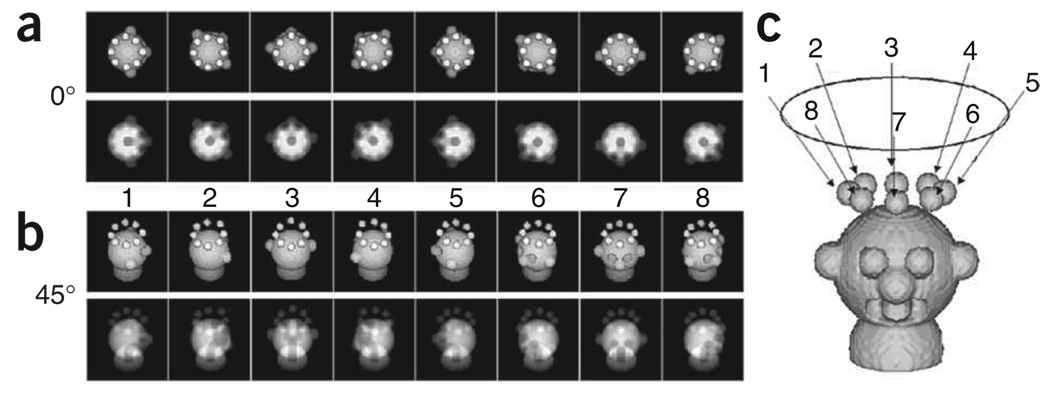
Geometry for collection of conical tilt data. (a) Surface views (top) and projections (bottom) of a hypothetical 0° view. (b) Surface views (top) and projections (bottom) of a 45° view. (c) Projection directions relative to the object in three dimensions.

Figure 2

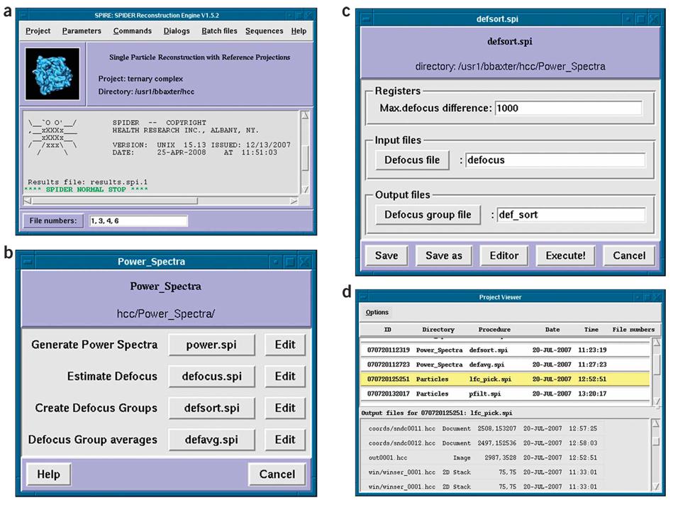
SPIRE. (a) SPIRE’s main window. (b) Dialog window with batch-file buttons. (c) The batch file form graphically presents the header values. (d) The Project Viewer.

Figure 3

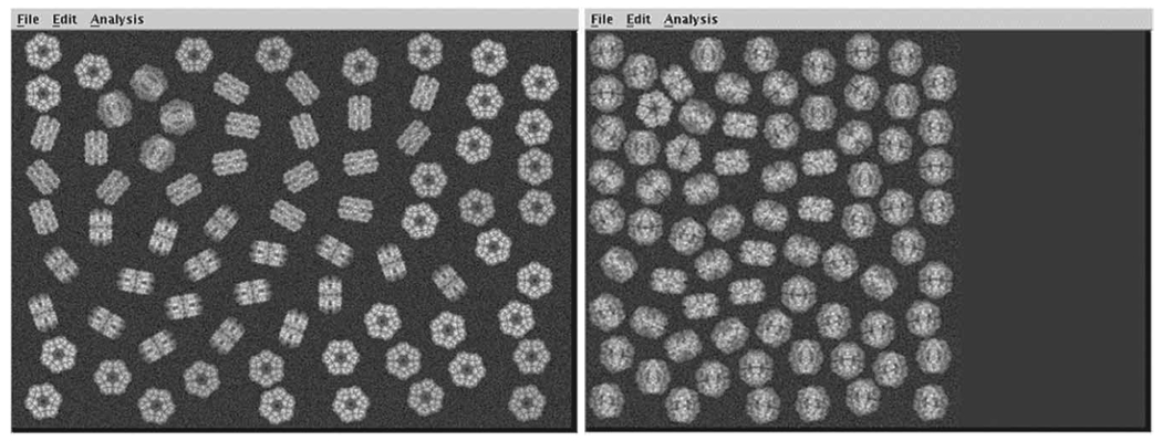
Simulated micrograph tilt pair. (Left) Untilted-specimen micrograph. (Right) Tilted-specimen micrograph.

Figure 4

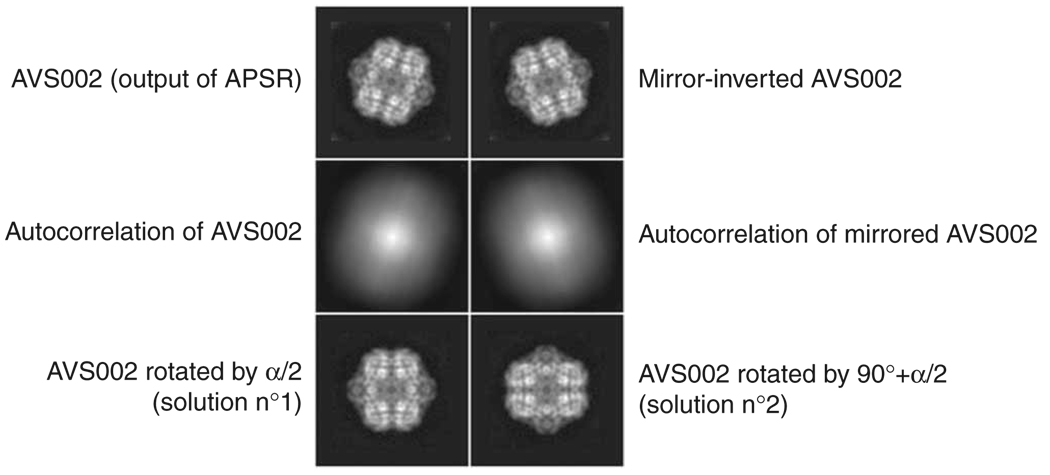
Reference-free alignment. Reorientation of the average from reference-free alignment along the coordinate axes. The first row of this montage shows the output file and its mirror-inverted copy. The second raw of the montage shows their respective autocorrelation functions. The last two images correspond to the two solutions of our alignment (α/2)° and (α/2) + 90°.

Figure 5

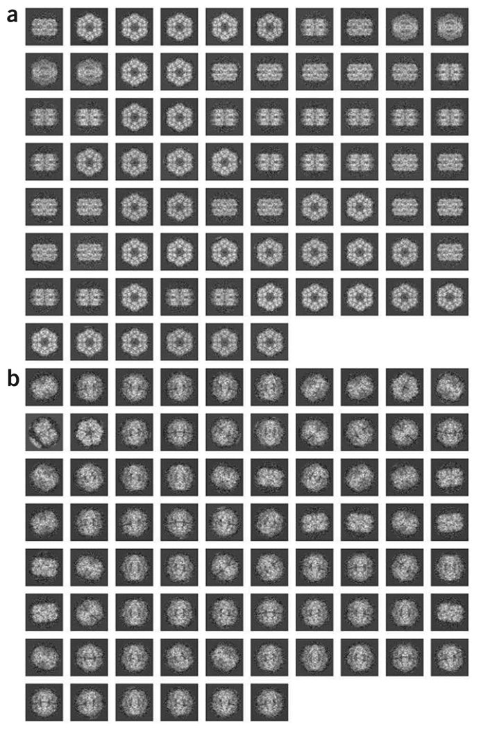
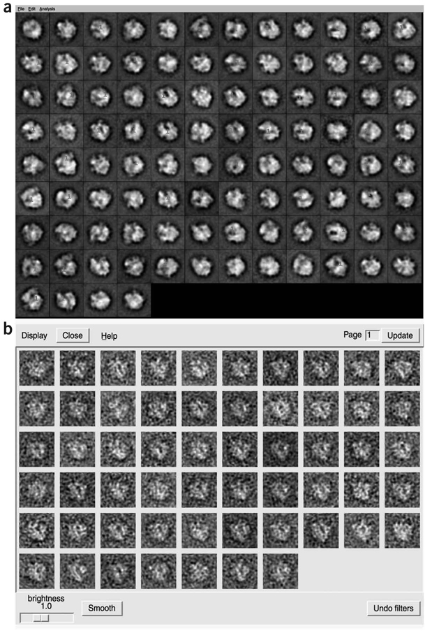
Windowed particles. (a) Montage of aligned, untilted particle images. (b) Montage of centered, tilted images.

Figure 6

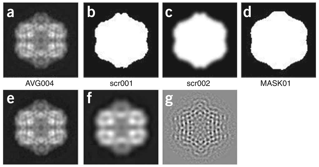
Creation of a binary mask and filtration. (a) Average image, from b06.fed. (b) Thresholded average. (c) Low-pass filtered. (d) Thresholded version of (c). (e) Original image, unfiltered. (f) Low-pass filtration at 1/35 Å⁻¹. (g) High-pass filtration at 1/25 Å⁻¹.

Figure 7

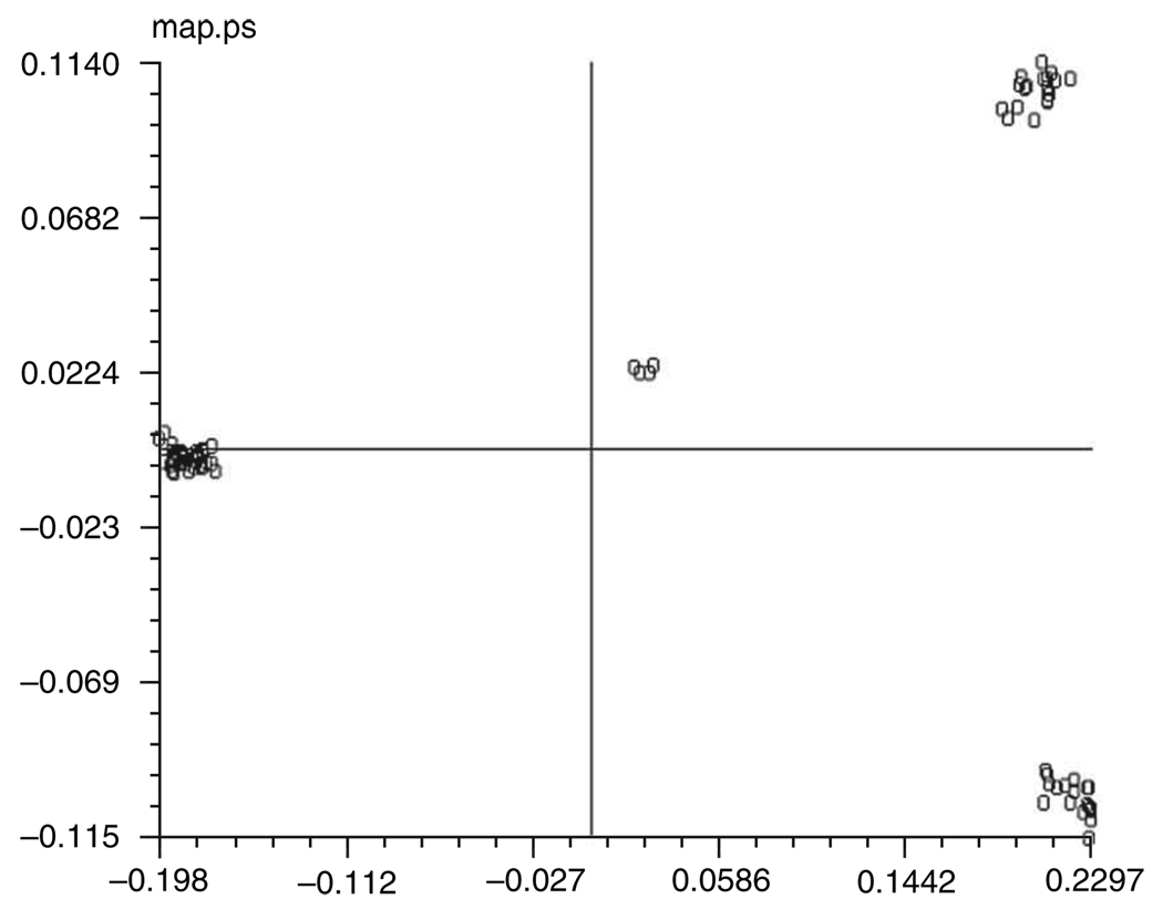
Factor map. Factor 1 is the abscissa. Factor 2 is the ordinate.

Figure 8

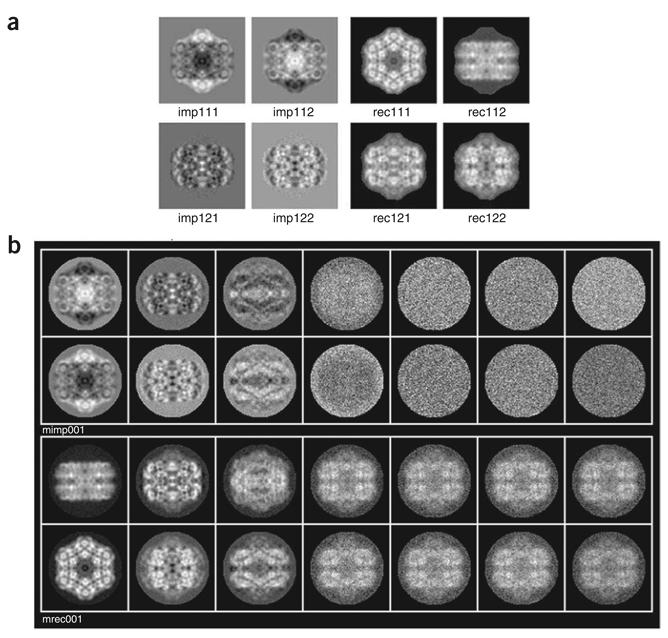
Importance and reconstituted images. (a) Importance (left) and reconstituted (right) images. (b) Montage of importance images (top) and reconstituted images (bottom). Note that factors 4–7 contain no information related to the variability of views but rather contain spurious noise.

Figure 9

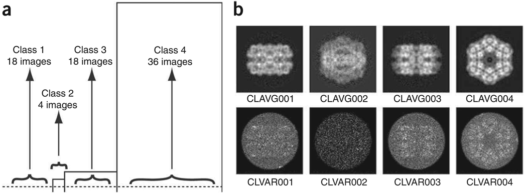
Clustering of images. (a) Truncated dendrogram. (b) Class averages (top) and class variances (bottom).

Figure 10

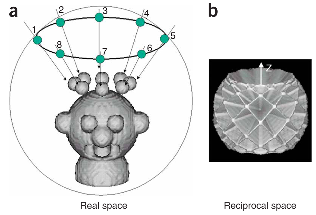
The missing-cone artifact. (a) Projection directions. (b) Illustration of the missing cone. In reciprocal space, every 2D projection of a 3D object corresponds to a central section in the 3D Fourier transform of the object. Each central section is orthogonal to the direction of the projection. A conical tilt series allows sampling of the 3D Fourier transform of the object in all directions, except in a cone along the z axis, hence the term missing-cone artifact.

Figure 11

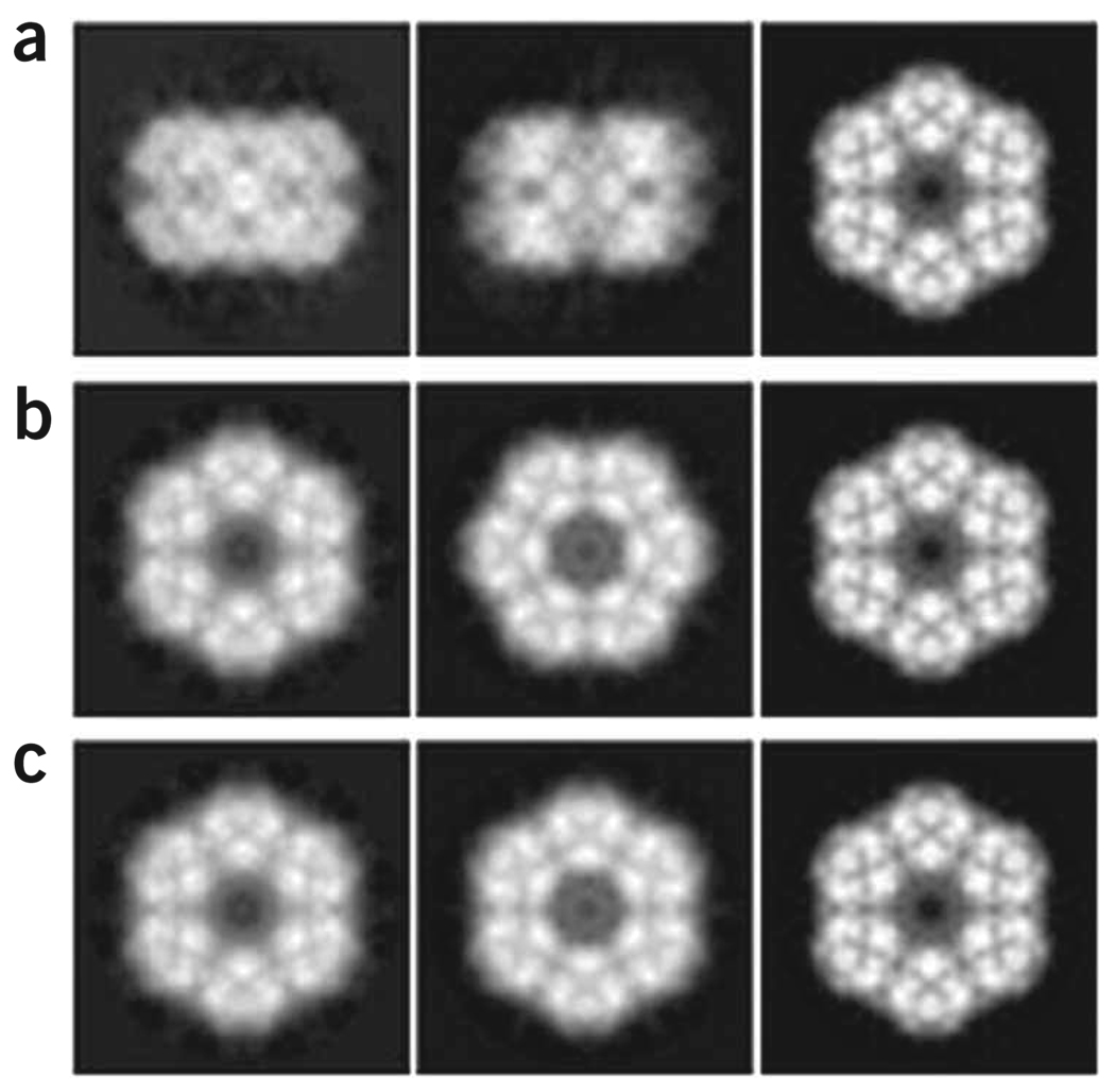
2D projections of 3D reconstructions for classes. (a) Projections along the z axis of reconstructions from classes 1, 3 and 4. (b) Projections after 90° rotation about the x axis for class reconstructions 1 and 3. (c) Projections after an additional rotation of 30° about the z axis for reconstruction 3.

Figure 12

Merged reconstruction. (a) Surface rendering, using UCSF Chimera, of the 3D reconstruction vtot001.hbl, generated below by batch file b15.fed. (b) Slice series through the merged reconstruction vtot001.hbl.

Figure 13

z slices through one of the two reconstructions used to generate phantom data.

Figure 14

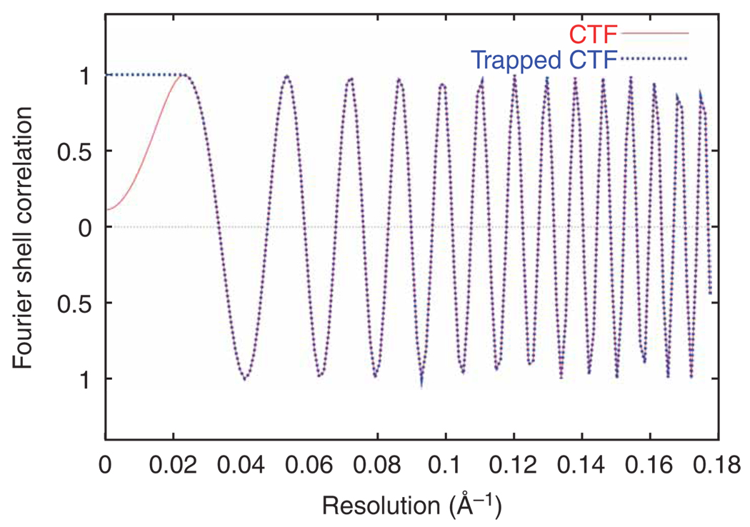
CTF profiles as a function of spatial frequency. The output of SPIDER command TF L is in red. The blue curve, which preserves low spatial frequencies, will be used. Note that beyond 0.02 Å⁻¹ the two profiles are the same, appearing as a purple line.

Figure 15

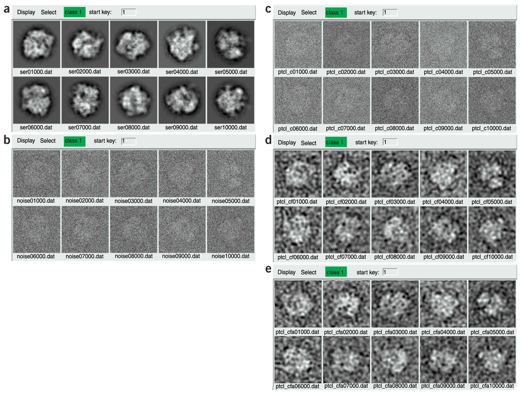
Processing of phantom data. (a) Noise-free projections of the input reconstructions. (b) Projections to which Gaussian-distributed noise has been added. (c) CTF-corrected projections. (d) Low-pass-filtered versions of projections in (c). (e) Images after reference-free alignment.

Figure 16

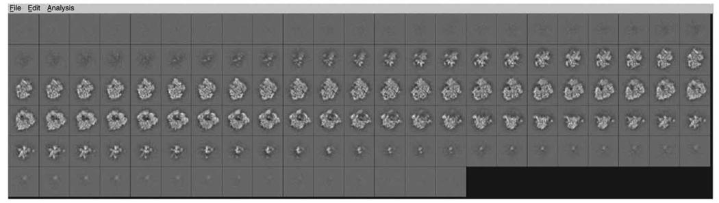
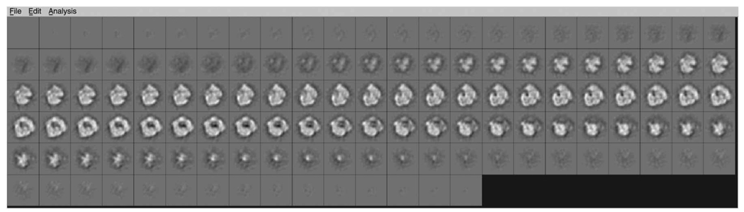
K-means classification. (a) Montage of class averages. Images with a green ‘1’ were selected for common-lines alignment. (b) Montage of filtered images assigned to the same class.

Figure 17

z slices through a common-lines reconstruction that closely resembles the correct solution.

Figure 18

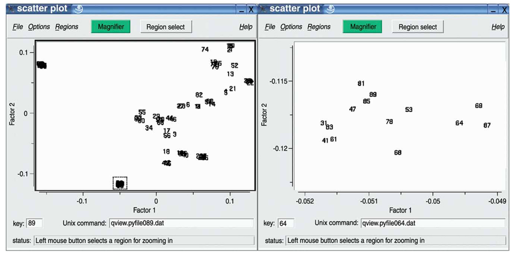
Scatter plot of factor 1 versus factor 2, generated with scatter.py. (left) and overview plot (right). Close-up view of boxed area in left. A PostScript version of factor 1 versus factor 2 is also generated by volmsa.cor.

Figure 19

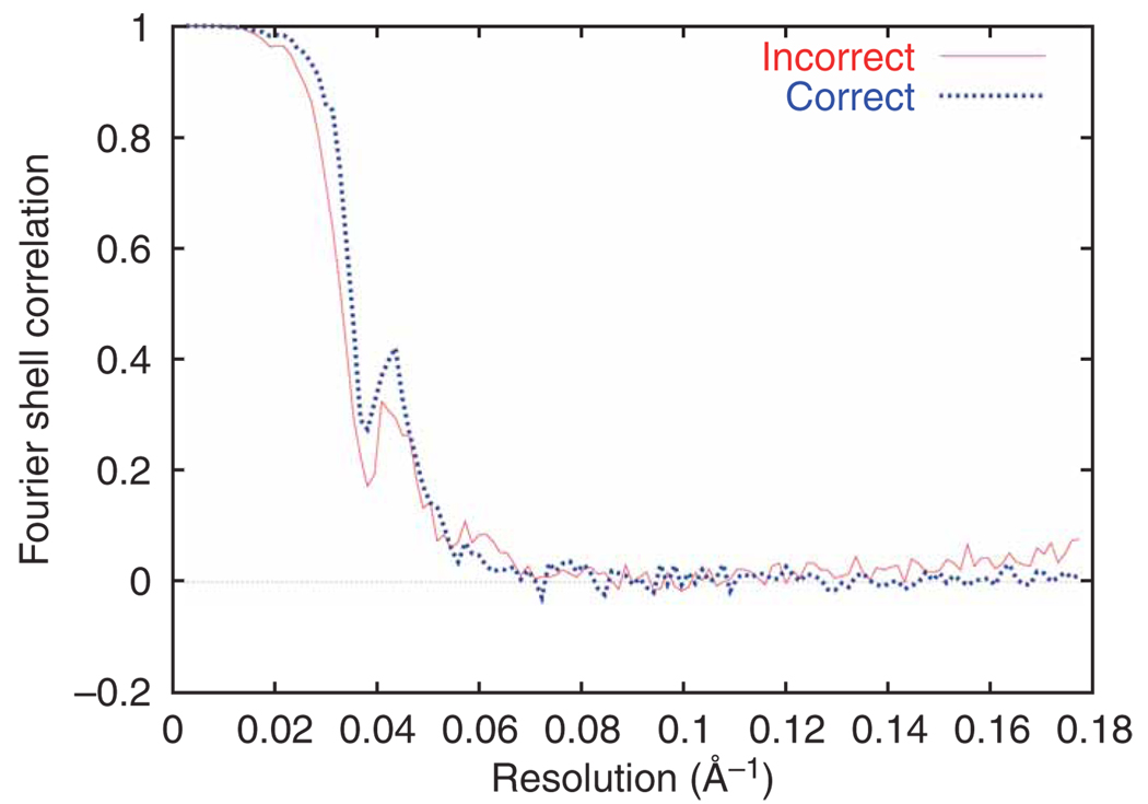
FSC curves after two iterations of refinement.

Figure 20

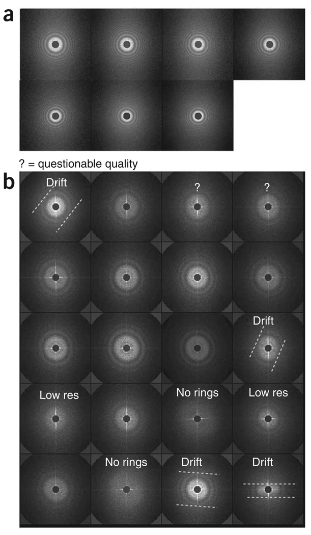
Power spectra. (a) A gallery of 2D power spectra (power/pw_avg***) of a series of micrographs with different defoci. The patterns of concentric rings are the Thon rings, which reflect the different CTFs. (b) A gallery of 2D power spectra with examples of problems. Question marks indicate power spectra that fall off rapidly after the first plateau.

Figure 21

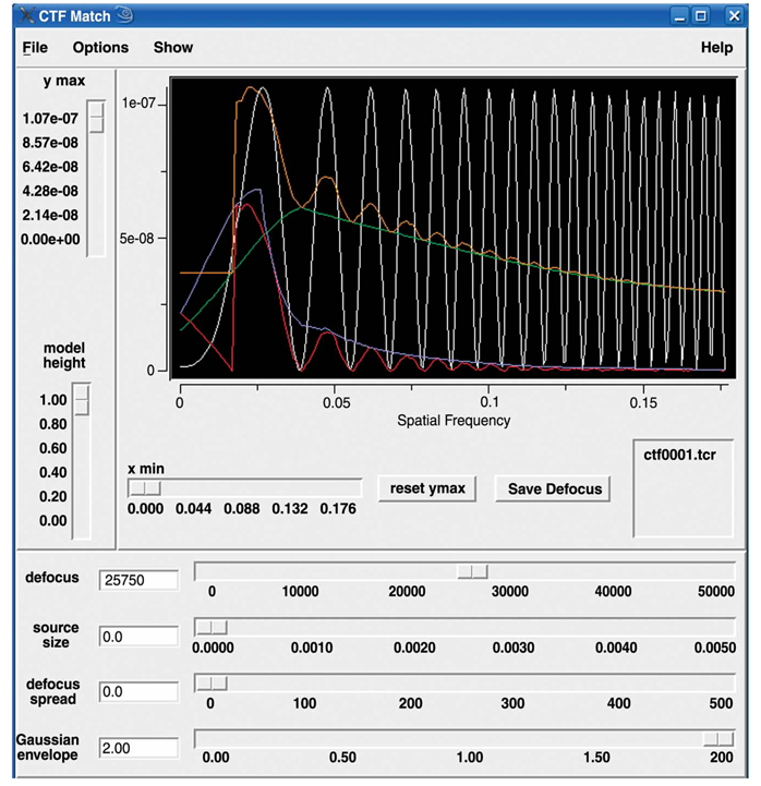
Manual fitting of a CTF model to a 1D power spectrum profile (power/roo***) using ctfmatch.py.

Figure 22

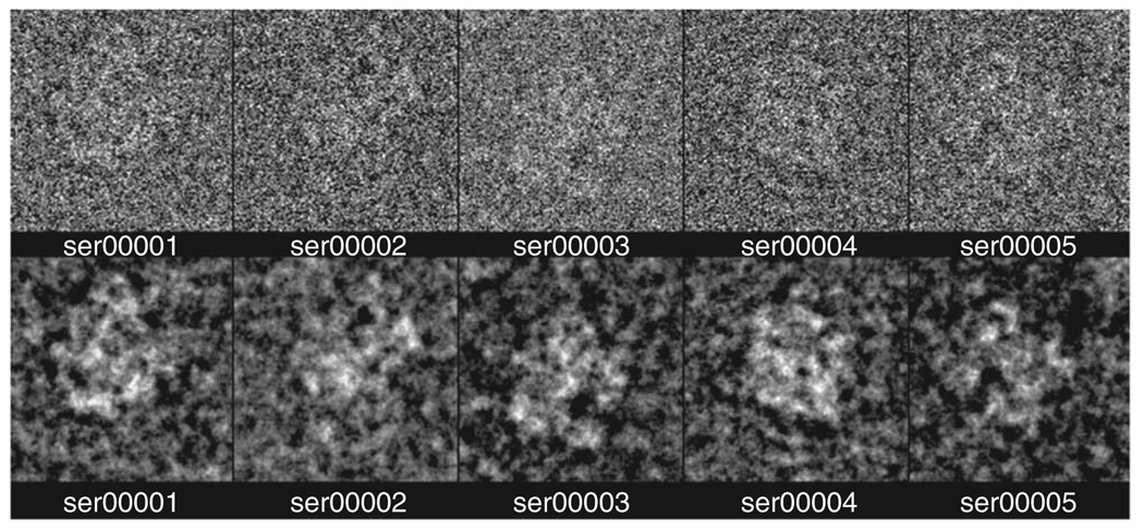
Examples of particle images before (top) and after filtering (bottom).

Figure 23

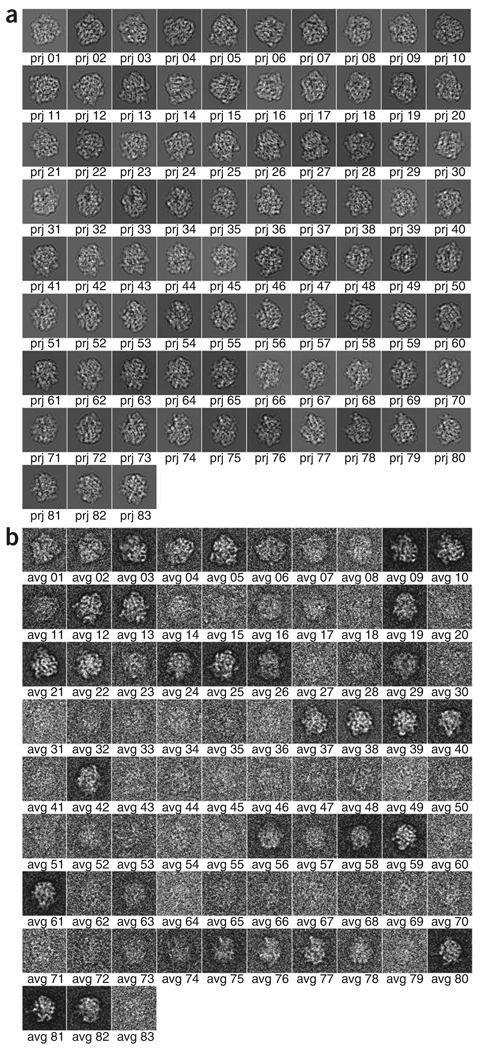
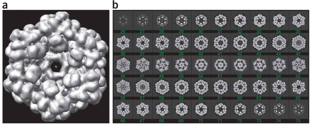
Multiple references. (a) Gallery of 83 projections of the reference. (b) Averaged particle images in a single defocus group.

Figure 24

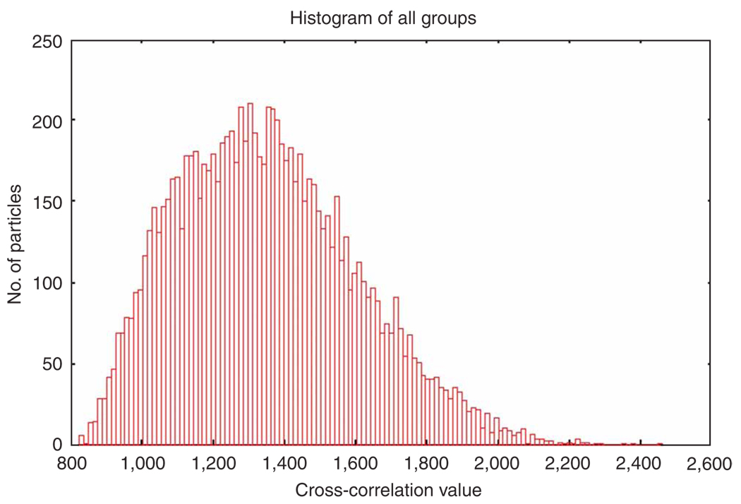
Correlation histogram of all particles.

Figure 25

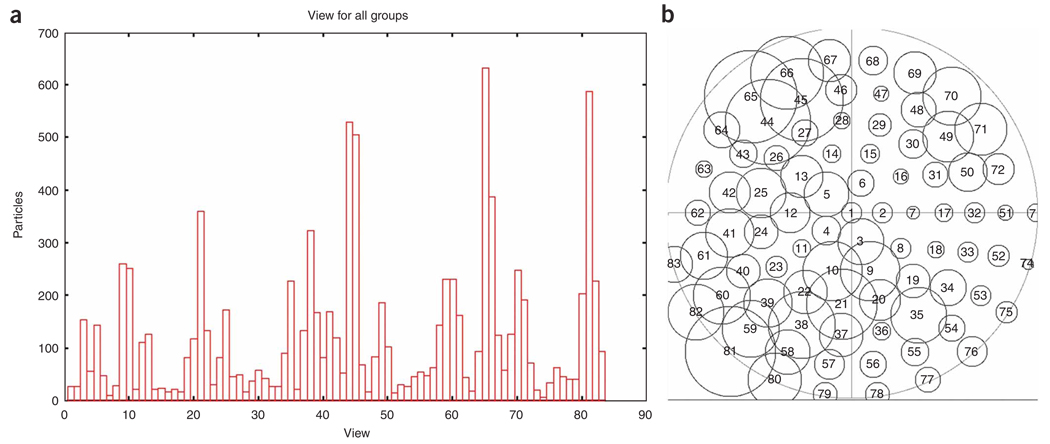
Distribution of orientations. (a) Histogram of number of particles versus projection view. (b) Map of angular coverage. Numbers in circles denote the Eulerian angles (ordered in a spiral outgoing from the pole); areas of circles are proportional to numbers of particle projections falling into that direction.

Figure 26

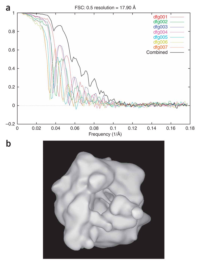
Initial reconstruction. (a) FSC curves for all defocus groups, and for the combined set. (b) Surface rendering of the initial reconstruction (map filtered at 17.9 Å).

Figure 27

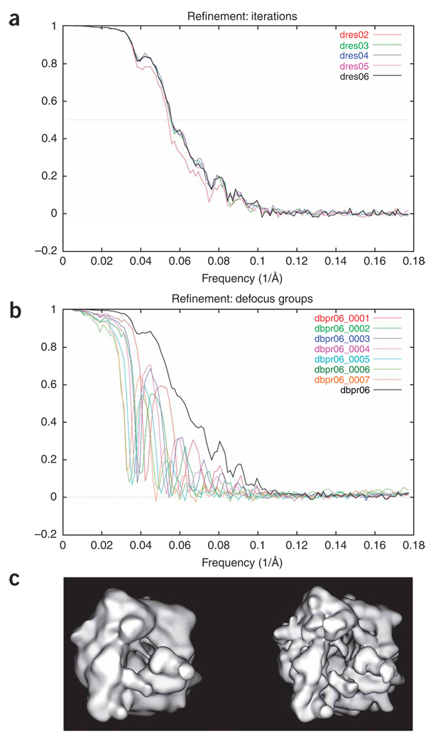
Refined reconstruction. (a) FSC curves for each iteration. (b) Refined (last iteration) FSC curve of each defocus group, along with the combined resolution curve. (c) Comparison of initial (left, 17.9 Å) and refined (right, 16.0 Å) reconstructions.

Figure 28

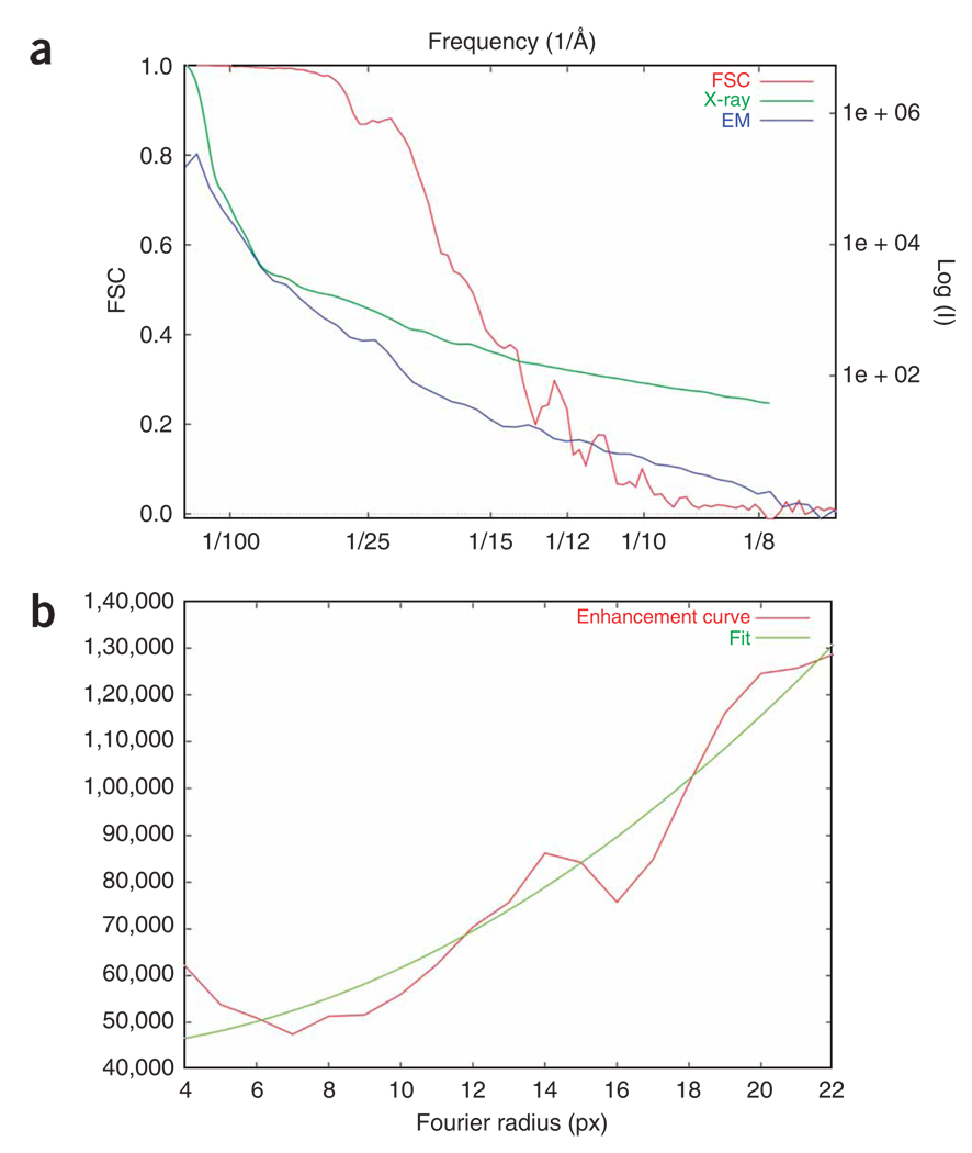
Amplitude-enhancement profiles. (a) Profiles of Fourier shell correlation, Fourier amplitudes of the EM map (bpr06.dat) and the low-angle X-ray solution scattering data. (b) Fitting of the enhancement curve.

Figure 29

Effect of amplitude enhancement. (a) Comparison of maps before (left) and after (right) the Fourier amplitude correction. (b) Effect of amplitude correction on a 9.9-Å EM map (reconstructed from the same data set described in this protocol, using original 91,114 particles).

Figure 30

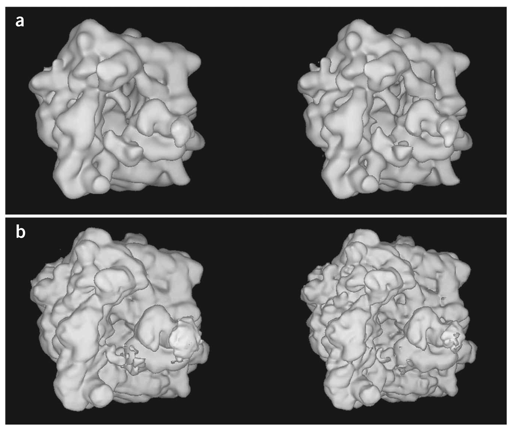
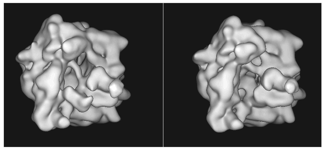
Reference maps used for supervised classification. These maps differ in the degree of ‘ratchet’ rotation of the 30 versus 50S subunit. (a) Unratcheted ribosome. (b) Ratcheted ribosome.

Figure 31

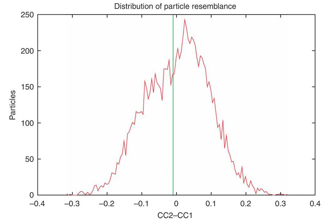
Distribution of particle resemblance with respect to the two references (red curve), which reveals a possible bimodel distribution. Here, the data set is divided into two subsets at ΔCC= −0.01 (green line).

Figure 32

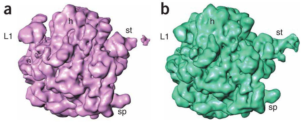
Reconstructions from two subsets using supervised classification. The map no. 1 (left) is reconstructed from subset no. 1 using 5,834 particles and map no. 2 (right) is reconstructed from subset no. 2 using 4,166 particles. In one of the maps, EF-G becomes visible as a solid mass, but it is absent in the other map. In contrast, the previous map generated from the entire dataset (Fig. 29a) contains EF-G as a fragmented, incomplete mass.

References

-
- Frank J. Three-Dimensional Electron Microscopy of Macromolecular Assemblies. New York: Oxford University Press; 2006.
- Glaeser RM, Downing K, DeRosier D, Chiu W, Frank J. Electron Crystallography of Biological Macromolecules. New York: Oxford University Press; 2007.
- Frank J, Shimkin B, Dowse H. SPIDER-a modular software system for electron image processing. Ultramicroscopy. 1981;6:343–358.
- Frank J, et al. SPIDER and WEB: processing and visualization of images in 3D electron microscopy and related fields. J. Struct. Biol. 1996;116:190–199. - PubMed
- van Heel M, Keegstra W. Imagic: a fast, flexible, and friendly image processing software system. Ultramicroscopy. 1981;7:113–129.
Publication types
MeSH terms
Grants and funding
LinkOut - more resources
Full Text Sources
Other Literature Sources