ANALYSIS OF HEPATITIS C VIRUS INFECTION MODELS WITH HEPATOCYTE HOMEOSTASIS

Abstract

Recently, we developed a model for hepatitis C virus (HCV) infection that explicitly includes proliferation of infected and uninfected hepatocytes. The model predictions agree with a large body of experimental observations on the kinetics of HCV RNA change during acute infection, under antiviral therapy, and after the cessation of therapy. Here we mathematically analyze and characterize both the steady state and dynamical behavior of this model. The analyses presented here are important not only for HCV infection but should also be relevant for modeling other infections with hepatotropic viruses, such as hepatitis B virus.

Fig. 1.1

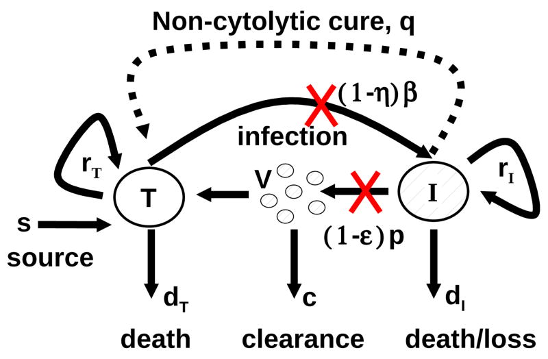
Schematic representation of HCV infection models. T and I represent target and infected cells, respectively, and V represents free virus. The parameters shown in the figure are defined in the text. The original model of Neumann et al. [37] assumed that there is no proliferation of target and infected cells (i.e., r_T = r_I = 0) and no spontaneous cure (i.e., q = 0). The extended model of Dahari et al. [6], which was used for predicting complex HCV kinetics under therapy, includes target and infected cell proliferation without cure (r_T, r_I > 0 and q = 0). A model including both proliferation and the spontaneous cure of infected cells(dashed line; q > 0) was used to explain the kinetics of HCV in primary infection in chimpanzees [5].

Fig. 2.1

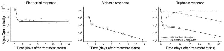
Three example plots of observed changes in viral load (X) following the start of treatment, together with numerical solutions to System (2.1) (solid line). The initial condition of each numerical solutions is the chronic-infection steady-state. In some cases, there is a flat partial response to treatment (left), where viral load shows an immediate drop, but then remains unchanged over time. In some cases, there is a biphasic response (middle), with a rapid initial drop and a slower asymptotic clearance. In some cases, there is a triphasic response, with a rapid initial drop, an intermediate shoulder phase during which there is little change, and then an asymptotic clearance phase. The initial rapid decline in virus load is the synchronization to the new quasi-steady state, following the start of treatment. Afterward, virus load closely tracks the number of infected cells (right). Treatment efficacies are ε = 0.98,η = 0 (left), ε = 0.9, η = 0 (middle), and ε = 0.996,η = 0 (right). Other parameter values are shown in Table 2.1.

Fig. 3.1

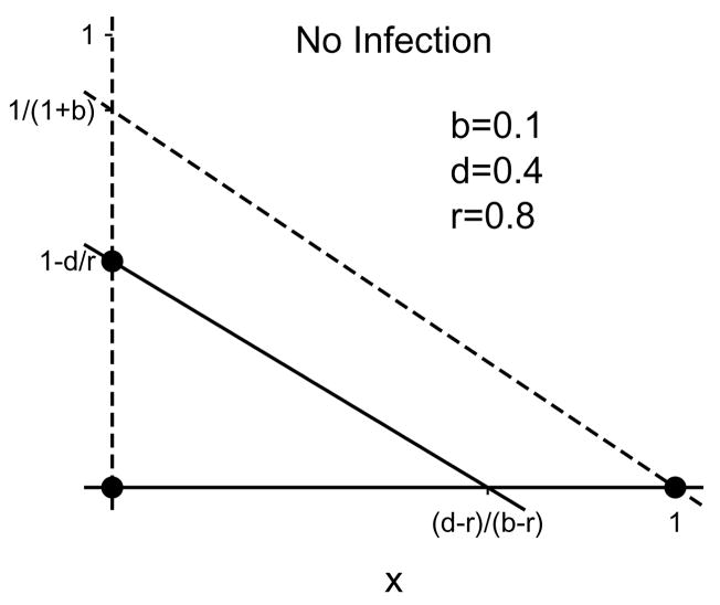
Example nullclines for System (2.8) when the disease-free equilibrium is globally attracting. The liver-free (x = y = 0), disease-free (x = 1, y = 0), and total-infection (x = 0, y = 1 − d/r) stationary solutions are marked with dots. The solid lines are the ẏ-nullclines, the dotted lines are the ẋ-nullclines. The partial-infection stationary solution is not present for these parameter values.

Fig. 3.2

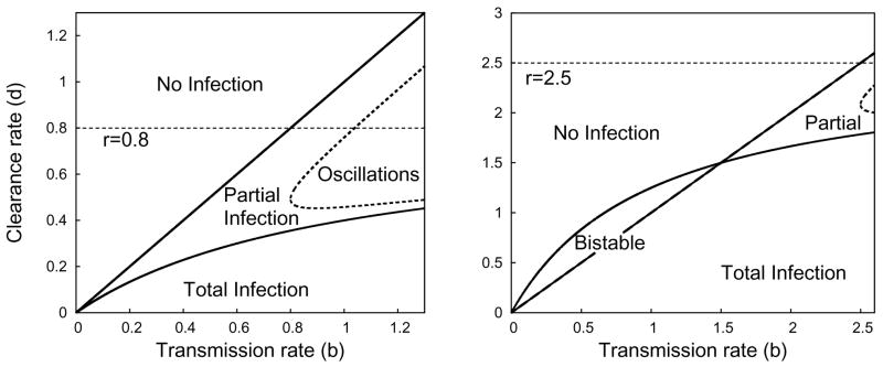
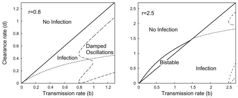
Plot representing the parameter regions for asymptotic dynamics of System (2.8) when r = 0.8 (left) or r = 2.5 (right). Within the region marked partial infection, the dotted line is the boundary between monotone convergence and oscillatory convergence to the partial infection steady state.

Fig. 3.3

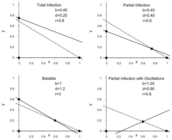
Example phase planes of System (2.8) for distinct parameter regions. The dashed lines are the ẋ-nullclines and the solid lines are the ẏ-nullclines. The dots represent stationary solutions.

Fig. 3.4

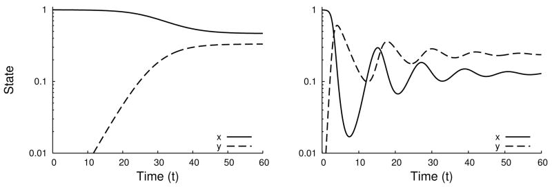
Time series for System (2.7) of monotone (left, r = 0.6, b = 0.6) and oscillatory (right, r = 0.1, b = 2.6) convergence to the partial infection stationary solution when d = 0.4.

Fig. 3.5

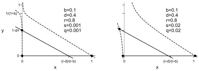
Example nullclines for System (2.7) when the disease-free equilibrium is globally attracting for immigration and spontaneous clearance rates s = q = 0.001 (left) or s = q = 0.02 (right). The liver-free, disease-free, and total-infection stationary solutions are marked with dots. The liver-free and total-infection stationary solutions have negative x coordinates when the immigration and spontaneous clearance rates are positive. The solid lines are the ẏ-nullclines, the dotted lines are the ẋ-nullclines. The partial-infection stationary solution is not present for these parameter values.

Fig. 3.6

Plot representing the parameter regions for asymptotic dynamics of System (2.7) with s = 0.01, q = 0 when r = 0.8 (left) or r = 2.5 (right). Compare to Figure 3.1. The dashed line represents the boundary of the parameter region where convergence to the steady state exhibits damped oscillations. The dotted line represents the bifurcation boundary between partial and total infection when s = q = 0. However, there is no formal bifurcation between partial and total infection if s or q is positive because of the structural instability of the transcritical bifurcation in System (2.8).

Fig. 4.1

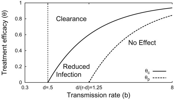
The treatment efficacy θ leading to specific dynamics for various transmission rates b, given d = 0.5, r = 0.9, s = 0 and q = 0. Treatment efficacies below θ_p have little or no effect on the number of infected hepatocytes. Treatment efficacies between θ_c and θ_p reduce the number of infected hepatocytes, but are not sufficient for complete clearance. Treatment efficacies greater than θ_c lead to complete clearance of infection.

Fig. 4.2

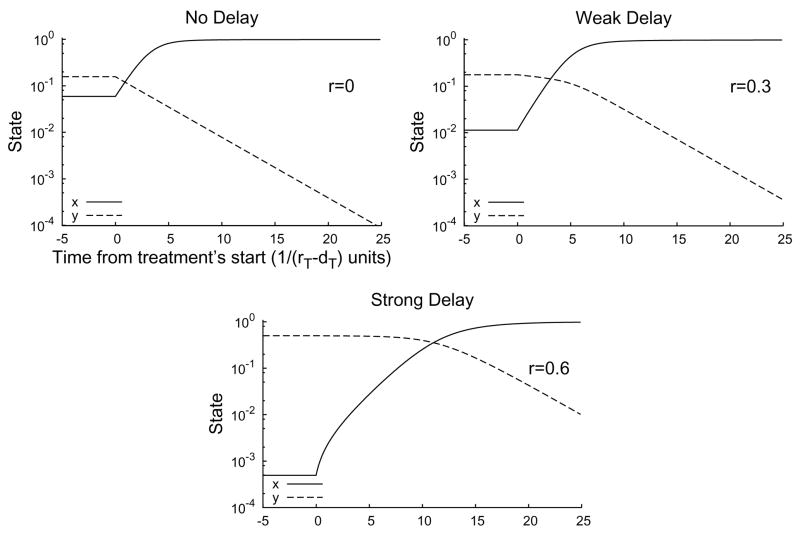
Time series for System (2.7) with treatment starting at t = 0 for r = 0 (top, left), r = 0.3 (top, right), and r = 0.6 (bottom). The initial condition is the pre-treatment stationary solution. When the proliferation rate r is small (top, left), there is no delay; the number of infected cells (y) decays at a constant rate from the start of treatment. For intermediate proliferation rates (top, right), there may is a weak delay between the start of treatment and the asymptotic clearance of infection. When r is large (bottom), there is a strong delay (about 10 units, here) before the number of uninfected cells (x) reaches equality with the number of infected cells and the number decay rate of infected cells accelerates to its exponential asymptotic rate. Parameter values s = 0.001, q = 0, d = 0.3, b = 5, θ = 1.

Fig. 4.3

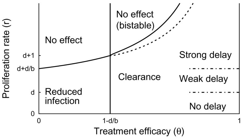
Classification of treatment-response as a function of θ and r when b > d. q = 0, s = 0.001, b = 0.9, d = 0.5. Regions are labelled according to the dynamics observed under treatment, assuming the dynamics were at equilibrium prior to treatment. In the bistable region, both the disease-free and total-infection stationary solutions are locally stable under treatment. The boundaries between the regions of strong delay, weak delay, and no delay are fuzzy, in the case of θ = 1, and the boundaries are even fuzzier for θ < 1. In the sliver between the dotted line and the solid line defining the bistable region our approximation to t_d in Eq. (4.8) fails because there is no nearby stationary solution to use for u* (see Fig. 4.4). In this sliver, the approximation method described in Appendix C can be used.

Fig. 4.4

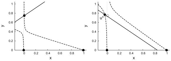
Nullclines of System (2.7) when s = 0.001, q = 0.008, r = 0.8, d = 0.2, and b = 1.5 with before treatment, θ = 0 (left) and at the start of treatment, θ = 14/15 (right). The solid dots represent stationary solutions. The open dot in the right-hand plot corresponds to the attracting stationary solution in the left-hand plot and is the initial condition for the dynamics when treatment begins. The adjacent solid dot u* is the unstable stationary solution around which we linearize to approximate the treatment delay.

Fig. 4.5

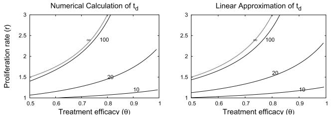
Side-by-side comparison of contour plots of the treatment t_d using numerical solution of system (2.7) (left) and the Formula (4.8) derived from the linear approximation (right). The approximate bound on bistability, $\text{r}=\text{d}+\frac{\text{d}}{(1-\theta )\text{b}}$, labeled ∞, is the same in both plots. Contour heights are 10, 20,100 and ∞. Parameter values d=0.5, b=1, s=10⁻³, q=0.θ_c=0.5 when r=0 in both plots.

Fig. 4.6

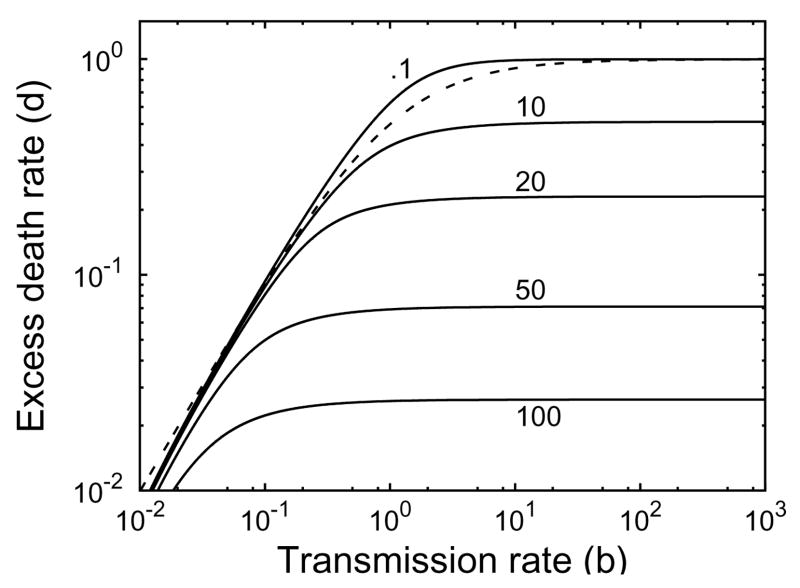
Contour plot of the treatment delay t_d from Eq. (4.8) as functions of d and b when r =1,θ = 1, s = 10⁻³ and q=0. Contours at .1, 10, 20, 50, and 100. The dotted line d = rb/(1+b) is an upper bound on the region of strong-delay effect.

Fig. 4.7

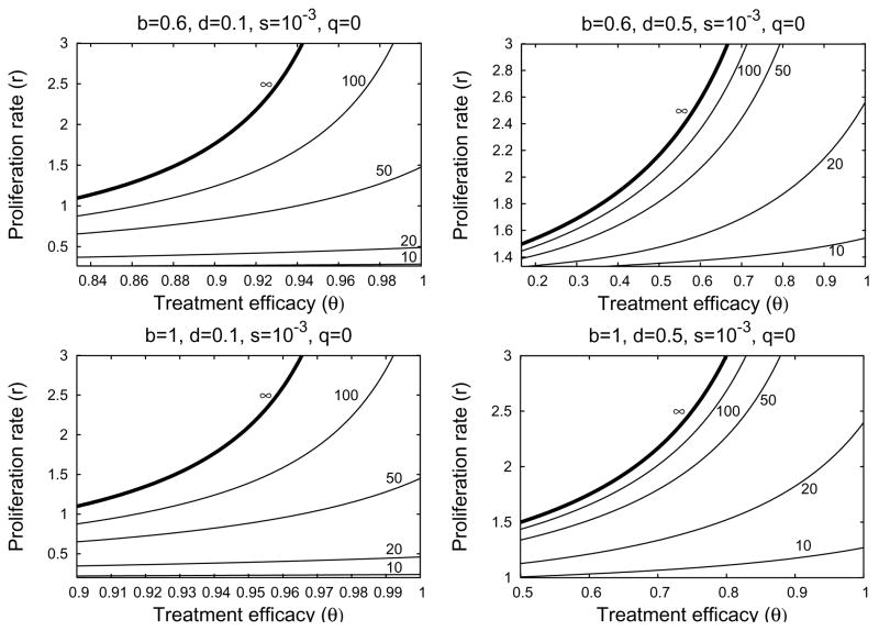
Four contour plots of treatment delay t_d in the strong-delay region of Figure 4.3, calculated from Formula (4.8) when hepatocyte immigration is slow. In the parameter region above the ∞-contour, treatment is not sufficiently effective to overcome the local stability of the infected-cell population. Below the ∞-contour, treatment successfully clears infection, with the length of the delay given by the contour values. Parameter values are given at the top of each plot. The left-hand boundary in each plot corresponds to θ = θ_C when r = 0.

Fig. 4.8

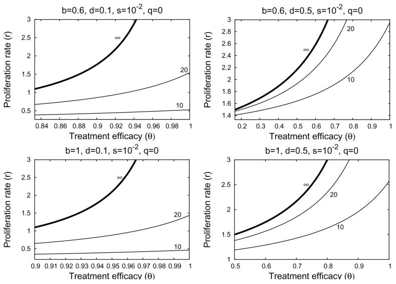
Four contour plots of treatment delay t_d in the strong-delay region of Figure 4.3, calculated from Formula (4.8). Parameter values are stated at the top of each plot. In the parameter region above the ∞-contour, treatment is not sufficiently effective to overcome the local stability of the infected-cell population. Below the ∞-contour, treatment successfully clears infection, with the length of the delay given by the contour values. In these plots, immigration is fast (s = 10⁻²) and significantly reduces the delay before treatment reduces the number of infected cells, compared to Figure 4.7. The left-hand boundary in each plot corresponds to θ = θ_C when r = 0.

Fig. 4.9

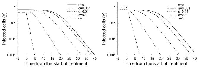
Time series plot of changes in the number of infected cells under treatment with s = 0.001 (left) and q = 0.001 (right). As the curing of infected cells q is increased from 0 to 1, the treatment delay decreases from 15 to 0 (left). Similarly, treatment delay decreases as the immigration rate s increases (right). Note that only vary large values of s and q significantly effect the pre-treatment state. Parameter values d = 0.3, b = 3,θ = 1, r = 1.

References

-
- Dahari H, Feilu A, Garcia-Retortillo M, Forns X, Neumann AU. Second hepatitis C replication compartment indicated by viral dynamics during liver transplantation. Journal of Hepatology. 2005;42:491–498. - PubMed
- Dahari H, Major M, Zhang X, Mihalik K, Rice CM, Perelson AS, Feinstone SM, Neumann AU. Mathematical modeling of primary hepatitis C infection: Noncytolytic clearance and early blockage of virion production. Gastroenterology. 2005;128:1056–1066. - PubMed
Grants and funding
LinkOut - more resources
Full Text Sources