PyMVPA: A Unifying Approach to the Analysis of Neuroscientific Data

Abstract

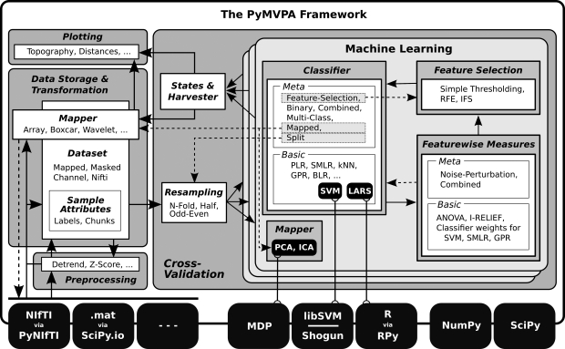
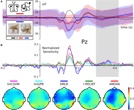
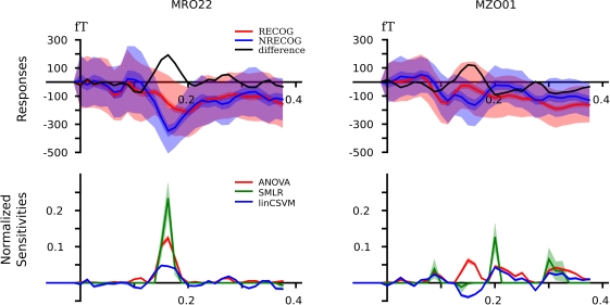
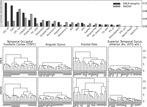
The Python programming language is steadily increasing in popularity as the language of choice for scientific computing. The ability of this scripting environment to access a huge code base in various languages, combined with its syntactical simplicity, make it the ideal tool for implementing and sharing ideas among scientists from numerous fields and with heterogeneous methodological backgrounds. The recent rise of reciprocal interest between the machine learning (ML) and neuroscience communities is an example of the desire for an inter-disciplinary transfer of computational methods that can benefit from a Python-based framework. For many years, a large fraction of both research communities have addressed, almost independently, very high-dimensional problems with almost completely non-overlapping methods. However, a number of recently published studies that applied ML methods to neuroscience research questions attracted a lot of attention from researchers from both fields, as well as the general public, and showed that this approach can provide novel and fruitful insights into the functioning of the brain. In this article we show how PyMVPA, a specialized Python framework for machine learning based data analysis, can help to facilitate this inter-disciplinary technology transfer by providing a single interface to a wide array of machine learning libraries and neural data-processing methods. We demonstrate the general applicability and power of PyMVPA via analyses of a number of neural data modalities, including fMRI, EEG, MEG, and extracellular recordings.

Keywords: Python; electroencephalography; extracellular recordings; functional magnetic resonance imaging; machine learning; magnetoencephalography.

Figure 1

PyMVPA workflow and design. PyMVPA is a modular framework. It consists of several components (gray boxes) such as ML algorithms or dataset storage facilities. Each component contains one or more modules (white boxes) providing a certain functionality, e.g., classifiers, but also feature-wise measures (e.g., I-RELIEF; Sun, 2007), and feature selection methods (recursive feature elimination, RFE; Guyon and Elisseeff, ; Guyon et al., 2002). Typically, all implementations within a module are accessible through a uniform interface and can therefore be used interchangeably, i.e., any algorithm using a classifier can be used with any available classifier implementation, such as support vector machine (SVM; Vapnik, 1995), or sparse multinomial logistic regression (SMLR; Krishnapuram et al., 2005). Some ML modules provide generic meta algorithms that can be combined with the basic implementations of ML algorithms. For example, a Multi-Class meta classifier provides support for multi-class problems, even if an underlying classifier is only capable to deal with binary problems. Additionally, most of the components in PyMVPA make use of some functionality provided by external software packages (black boxes). In the case of SVM, classifiers are interfaced to the implementations in Shogun or LIBSVM. PyMVPA only provides a convenience wrapper to expose them through a uniform interface. By providing simple, yet flexible interfaces, PyMVPA is specifically designed to connect to and use externally developed software. Any analysis built from those basic elements can be cross-validated by running them on multiple dataset splits that can be generated with a variety of data resampling procedures (e.g., bootstrapping, Efron and Tibshirani, 1993). Detailed information about analysis results can be queried from any building block and can be visualized with various plotting functions that are part of PyMVPA, or can be mapped back into the original data space and format to be further processed by specialized tools (i.e., to create an overlay volume analogous to a statistical parametric mapping). The solid arrows represent a typical connection pattern between the modules. Dashed arrows refer to additional compatible interfaces which, although potentially useful, are not necessarily used in a standard processing chain.

Figure 2

Sensitivities for the classification of color and line-art conditions. Panel (A) shows ERPs of each condition for electrode Pz. The light shaded area shows the standard deviation, the darker shade the 95% confidence interval around the mean ERP of each condition. The black curve is the difference wave of both ERPs. The stimulus example images are from Fründ et al. (2008). Panel (B) shows feature sensitivity measures for the different methods. Sensitivities were normalized by scaling the vector norm of each sensitivity vector (covering all timepoints from all electrodes) to unit length. This allows for comparison of the relative weight each classifier puts on each feature. The head topography plots in the lower panel show the channel-wise sum over time of the absolute scaled sensitivities. The upper panel shows the same scaled sensitivities plotted over time for the Pz electrode (indicated as the dark dot on the head topographies). This electrode was chosen as Fründ et al. (2008) made it the subject of most visualizations. The shape of the sensitivity curves nicely resemble the ERP difference wave. Interestingly, for a time window around 350 ms after stimulus onset (indicated by the gray bar), all multivariate sensitivity measures assign a considerable amount of weight on the respective timepoints, whereas the univariate ANOVA is completely flat at zero.

Figure 3

Event-related magnetic fields (EMF) and classifier sensitivities. The upper part shows EMFs for two exemplary MEG channels. On the left sensor MRO22 (right occipital), and on the right sensor MZO01 (central occipital). The lower part shows classifier sensitivities and ANOVA F-scores plotted over time for both sensors. Both classifiers showed equivalent generalization performance of approximately 82% correct single trial predictions.

Figure 4

Sensitivity analysis of the four-category fMRI dataset. The upper part shows the ROI-wise scores computed from SMLR classifier weights and ANOVA F-scores (limited to the 20 highest and the three lowest-scoring ROIs). The lower part shows dendrograms with clusters of average category samples (computed using squared Euclidean distances) for voxels with non-zero SMLR-weights and a matching number of voxels with the highest F-scores in each ROI.

Figure 5

Statistics of multiple single unit extracellular simultaneous recordings and corresponding classifier sensitivities. All plots sweep through different stimuli along vertical axis, with stimuli labels presented in the middle of the plots. The upper part shows basic descriptive statistics of spike counts for each stimulus per each time bin (on the left) and per each unit (on the right). Such statistics seem to lack stimulus specificity for any given category at a given time point or unit. The lower part on the left shows the temporal sensitivity profile of a representative unit for each stimulus. It shows that stimulus specific information in the response can be coded primarily temporally (few specific offsets with maximal sensitivity like for song2 stimulus) or in a slowly modulated pattern of spikes counts (see 3 kHz stimulus). Associated aggregate sensitivities of all units for all stimuli in the lower right figure indicate each unit's specificity to any given stimulus. It provides better specificity than simple statistics like variance, e.g., unit 19 is active in all stimulation conditions according to its high variance, but according to its classifier sensitivity it carries little, if any, stimuli-specific information for natural songs 1–3.

Figure 6

Confusion matrix of SMLR classifier predictions of stimulus conditions from of multiple unit recordings. The classifier was trained to discriminate between stimuli of five pure tones and five natural sounds. Elements of the matrix (numeric values and color-mapped visualization) show the number of trials which were correctly (diagonal) or incorrectly (off-diagonal) classified by a SMLR classifier during an eightfold cross-validation procedure. The results suggest a high similarity in the spiking patterns for stimuli of low-frequency pure tones, which lead the classifier to confuse them more often, whenever responses to natural sound stimuli and high-frequency tones were hardly ever confused with each other.

References

1. Beckmann C. F., Smith S. M. (2005). Tensorial extensions of independent component analysis for multisubject fMRI analysis. Neuroimage 25, 294–311 10.1016/j.neuroimage.2004.10.043 - DOI - PubMed
1. Birbaumer N., Cohen L. G. (2007). Brain-computer interfaces: communication and restoration of movement in paralysis. J. Physiol. 579, 621–636 10.1113/jphysiol.2006.125633 - DOI - PMC - PubMed
1. Busch N. A., Herrmann C. S., Müller M. M., Lenz D., Gruber T. (2006). A cross-laboratory study of event-related gamma activity in a standard object recognition paradigm. Neuroimage 33, 1169–1177 10.1016/j.neuroimage.2006.07.034 - DOI - PubMed
1. Detre G., Polyn S. M., Moore C., Natu V., Singer B., Cohen J., Haxby J. V., Norman K. A. (2006). The Multi-Voxel Pattern Analysis (MVPA) Toolbox. Poster presented at the Annual Meeting of the Organization for Human Brain Mapping (Florence, Italy). Available at: http://www.csbmb.princeton.edu/mvpa
1. Eads D. (2008). Hcluster: Hierarchical Clustering for SciPy. Available at: http://scipy-cluster.googlecode.com/
LinkOut - more resources