. 2009 Jun;46(2):432-46.
doi: 10.1016/j.neuroimage.2009.02.009. Epub 2009 Feb 20.

T1 weighted brain images at 7 Tesla unbiased for Proton Density, T2* contrast and RF coil receive B1 sensitivity with simultaneous vessel visualization

Affiliations

T1 weighted brain images at 7 Tesla unbiased for Proton Density, T2* contrast and RF coil receive B1 sensitivity with simultaneous vessel visualization

Pierre-François Van de Moortele et al. Neuroimage. 2009 Jun.

Abstract

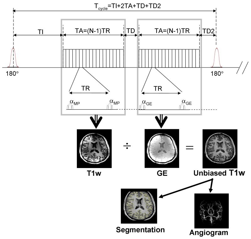
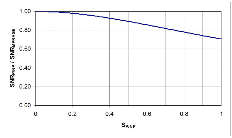
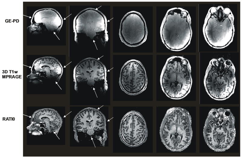
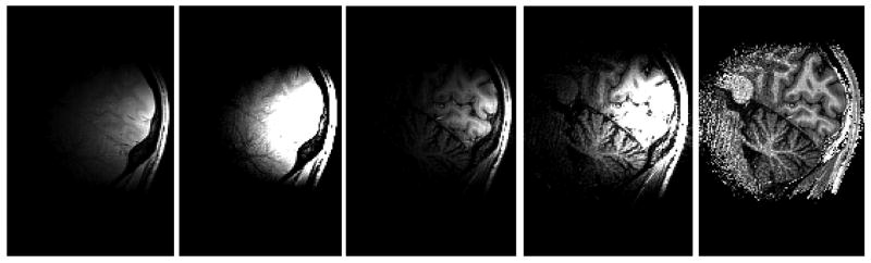
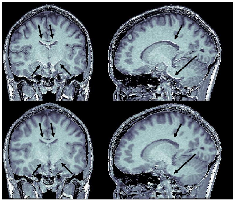
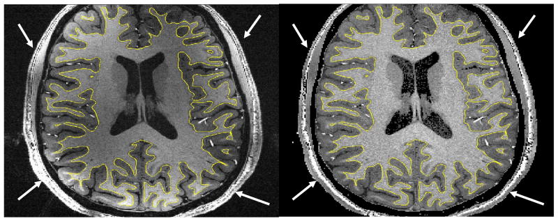
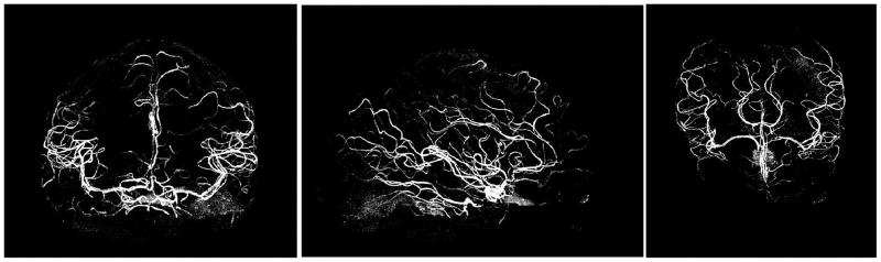
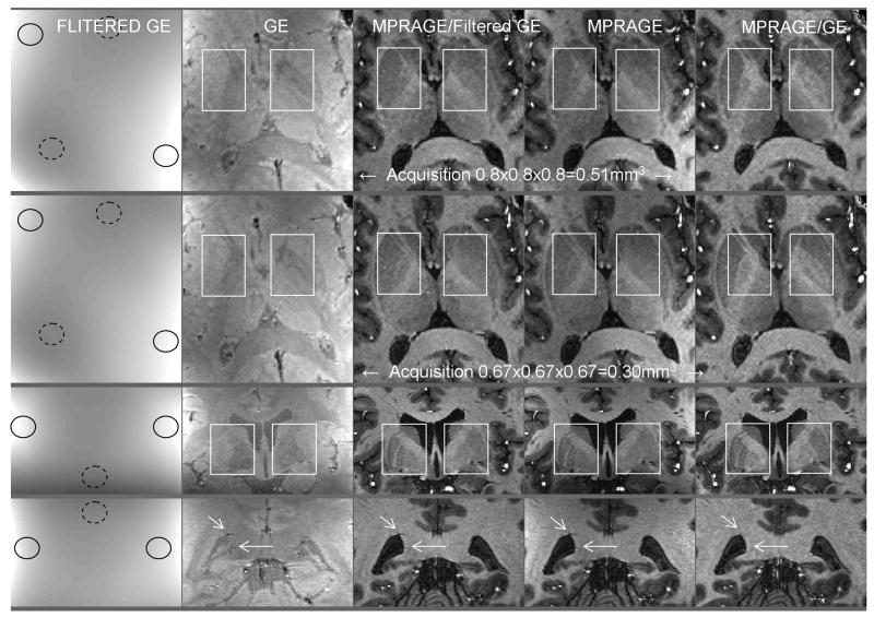
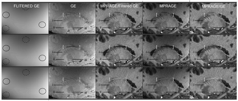
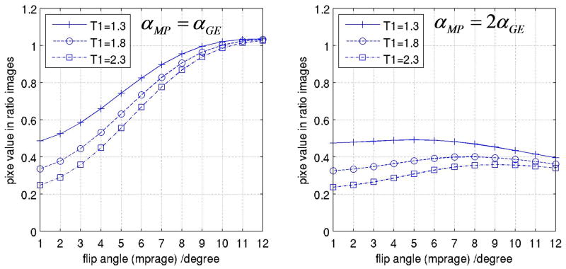
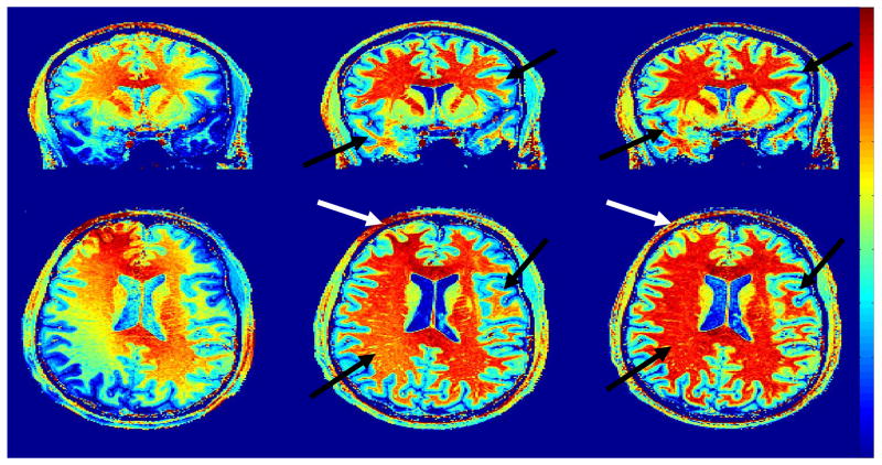
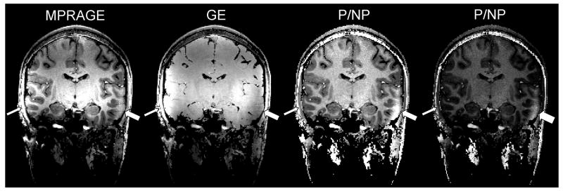
At high magnetic field, MR images exhibit large, undesirable signal intensity variations commonly referred to as "intensity field bias". Such inhomogeneities mostly originate from heterogeneous RF coil B(1) profiles and, with no appropriate correction, are further pronounced when utilizing rooted sum of square reconstruction with receive coil arrays. These artifacts can significantly alter whole brain high resolution T(1)-weighted (T(1)w) images that are extensively utilized for clinical diagnosis, for gray/white matter segmentation as well as for coregistration with functional time series. In T(1) weighted 3D-MPRAGE sequences, it is possible to preserve a bulk amount of T(1) contrast through space by using adiabatic inversion RF pulses that are insensitive to transmit B(1) variations above a minimum threshold. However, large intensity variations persist in the images, which are significantly more difficult to address at very high field where RF coil B(1) profiles become more heterogeneous. Another characteristic of T(1)w MPRAGE sequences is their intrinsic sensitivity to Proton Density and T(2)(*) contrast, which cannot be removed with post-processing algorithms utilized to correct for receive coil sensitivity. In this paper, we demonstrate a simple technique capable of producing normalized, high resolution T(1)w 3D-MPRAGE images that are devoid of receive coil sensitivity, Proton Density and T(2)(*) contrast. These images, which are suitable for routinely obtaining whole brain tissue segmentation at 7 T, provide higher T(1) contrast specificity than standard MPRAGE acquisitions. Our results show that removing the Proton Density component can help in identifying small brain structures and that T(2)(*) induced artifacts can be removed from the images. The resulting unbiased T(1)w images can also be used to generate Maximum Intensity Projection angiograms, without additional data acquisition, that are inherently registered with T(1)w structural images. In addition, we introduce a simple technique to reduce residual signal intensity variations induced by transmit B(1) heterogeneity. Because this approach requires two 3D images, one divided with the other, head motion could create serious problems, especially at high spatial resolution. To alleviate such inter-scan motion problems, we developed a new sequence where the two contrast acquisitions are interleaved within a single scan. This interleaved approach however comes with greater risk of intra-scan motion issues because of a longer single scan time. Users can choose between these two trade offs depending on specific protocols and patient populations. We believe that the simplicity and the robustness of this double contrast based approach to address intensity field bias at high field and improve T(1) contrast specificity, together with the capability of simultaneously obtaining angiography maps, advantageously counter balance the potential drawbacks of the technique, mainly a longer acquisition time and a moderate reduction in signal to noise ratio.


Figures

Fig. 1
Fig. 1. Interleaved 3D-MPRAGE and 3D-GE Sequence diagram
The first part of the sequence is a standard 3D MPRAGE, with a train of N small flip angle RF pulses (α) following each adiabatic inversion RF pulse (180°). TI=inversion time, TA=duration of the fast gradient echo train, TR=repetition time during the fast gradient echo trains, TD=optional delay. The interleaved version includes the second part which consists in repeating the fast gradient echo train (with all parameters identical expect for optional variations between αMP and αGE) followed by an optional delay TD2 immediately preceding the next inversion pulse (TD2 typically is zeroed). This cycle is repeated along the loop of the 3rd k-space dimension. αMP and αGE are the small flip angle during the fast echo train of MPRAGE and GE.
Fig. 2
Fig. 2. SNR in P/NP maps as a function of SNR in MPRAGE images
Ratio of Signal to Noise Ratio (SNR) in P/NP maps (SNRP/NP) over SNR in MPRAGE images (SNRMPRAGE) as a function of Signal Intensity in P/NP maps (SP/NP). Typical values for SP/NP are about 0.65 for white matter and 0.35 for gray matter, with corresponding relative loss in SNR of ∼16% and ∼6% respectively.
Fig. 3
Fig. 3. Whole Brain T1w Imaging at 7 Tesla (α = 3°)
Sagittal, coronal and axial views from a 3D Isotropic (1×1×1mm3) data set at 7Tesla. Top row: 3D GE-PD Middle row:3D MPRAGE Bottom row: P/NP ratio. White arrows indicate areas brighter or darker in MPRAGE and GE images which do not exhibit such regional intensity variation in ratio images. For some of those areas, such as cerebellum or anterior frontal lobe, identifying gray/white matter contrast without correction can be difficult. MPRAGE and GE-PD images were acquired separately with following acquisition parameters: TISiemens=1.5ss (MPRAGE only), TD=1.3s (MPRAGE only), TA= 1.34s, nominal flip angle: 3°. Scan times: 10min45s (MPRAGE) and 5min45s (GE). Note that GE-PD images are clearly dominated with Proton Density contrast (gray matter brighter than white matter). No motion correction was needed with this particular data set.
Fig. 4
Fig. 4. Surface Coil data at 7 Tesla
Sagittal view of GE-PD (two leftmost images), MPRAGE (next two images to the right) and P/NP map (single rightmost image) obtained from a 3D isotropic data set (1×1×1mm3 spatial resolution) in the occipital lobe at 7 Tesla. Whereas a single gray scale is sufficient to show the whole range of signal in the rightmost P/NP image, it is necessary to display the same image with two different gray scales for both GE-PD and MPRAGE in order to visualize the full range of tissues from darkest to brightest areas. Note the tremendous improvement in gray/white matter visibility in the rightmost P/NP map with high T1 contrast. The better noise visibility in low SNR areas should not be interpreted as noise amplification (see Methods). Images were acquired separately with standard MPRAGE and GE sequence: TISiemens=1.5s (MPRAGE only), TD=0.94s (MPRAGE only), TA= 1.12s, nominal flip angle: 3°. Scan time: 6min26s (MPRAGE) and 2min25s (GE).
Fig. 5
Fig. 5. Head Motion
P/NP ratio images without and with head motion correction. Corresponding MPRAGE and GE images were acquired with 0.65×0.65×1.5mm3 voxel size. Scan time was 10min49s for MPRAGE and 8min8s for GE. MPRAGE image was realigned onto GE image with the FLIRT package (see Methods). Top row: coronal and parasagittal views of P/NP ratio formed with uncorrected MPRAGE and GE images. Note the numerous edge artifacts (brighter edges are easier to identify than darker edges), some of them signaled with arrows. Bottom row: coronal and parasagittal views of the ratio between realigned MPRAGE and GE. The edge artifacts are not visible anymore (see arrows).
Fig. 6
Fig. 6. Brain segmentation with high resolution data
Axial view of 3D-MPRAGE (left) and of corresponding P/NP ratio (right) images from isotropic 3D data sets (0.65×0.65×0.65=0.27mm3 spatial resolution) obtained at 7T. 3D-MPRAGE (left) and 3D-GE (not shown) images were simultaneously acquired with the double contrast interleaved sequence with GRAPPA R=2 along the Y axis (TISiemens=1.5s, Tcycle=4.1s, TR=11.4ms, total scan time 14min12s). With non corrected 3D-MPRAGE volume (left) the SurfRelax package failed, even after spatial smoothing, to perform whole brain segmentation because of large signal inhomogeneities. The same procedure applied on P/NP ratio (right) resulted, even without spatial smoothing, in reliable gray/white matter segmentation (yellow contour overlaid on both images). Both images are deliberately shown without spatial filtering. Signal variations in the skin are also largely reduced in P/NP ratio (right) (see arrows), facilitating skin and skull striping procedures. The field of view is truncated along Y axis because of matrix size limits in our current implementation of the segmentation software.
Fig. 7
Fig. 7. Maximum Intensity Projection angiogram
Coronal, sagittal and axial projection (from left to right) of Maximum Projection Intensity angiogram obtained at 7 Tesla from P/NP ratio images. Corresponding 3D MPRAGE and 3D GE isotropic data sets (0.65×0.65×0.65=0.27mm3 spatial resolution) were obtained with the interleaved double contrast sequence, with GRAPPA R=2 along Y axis (TISiemens=1.5s, Tcycle=4.1s, TR=11.4ms, total scan time 14min12s). Before forming the ratio, both MPRAGE and GE images were zerofilled, and then GE images were smoothed with a 3D Gaussian kernel (∼1.5mm FWHM). Skin and skull as well as other non cerebral structures were removed with 3D morphomathematical tools and an intensity threshold was used to retain vessels pixels.
Fig. 8
Fig. 8. Low resolution versus matching high resolution reference image (I)
Axial (upper two rows) and coronal (lower two rows) views from high resolution 3D MPRAGE (fourth column) and 3D GE (second column) images acquired with the interleaved sequence. The first column shows GE images convolved with a 27.5×27.5mm2 FWHM Gaussian filter. Plain (dashed) circles signal areas of higher (lower) signal intensity due to receive B1 profile. Ratio images shown in third (fifth) column were obtained by dividing MPRAGE with the filtered (unfiltered) GE images. White boxes and arrows: see text in Result section. Acquisition parameters. Upper row: voxel size 0.8 × 0.8 × 0.8 = 0.51mm3, GRAPPA R=3, Partial Fourier [X,Y] = [6/8,6/8], TISiemens=1.5s, Tcycle=5.644s, TR=9.8ms, TE=4.45ms, bandwidth=140Hz/pixel, total scan time=7min12s. Second to fourth row: voxel size 0.67 × 0.67 × 0.67 = 0.30mm3, GRAPPA R=3, Partial Fourier [X,Y] = [6/8,6/8], TISiemens=1.5s, Tcycle=5.843s, TR=9.8ms, TE=4.45ms, bandwidth=140Hz/pixel, total scan time=11min24s.
Fig. 9
Fig. 9. Low resolution versus matching high resolution reference image (II)
Three contiguous parasagittal views (one per row) from high resolution 3D MPRAGE (fourth column) and 3D GE (second column) images acquired with the interleaved sequence. The first column shows GE images convolved with a 27.5×27.5mm2 FWHM Gaussian filter. Plain (dashed) circles signal areas of higher (lower) signal intensity due to receive B1 profile. Ratio images shown in third (fifth) column were obtained by dividing MPRAGE with the filtered (unfiltered) GE images. White brackets and labels: see text in Result section. Acquisition parameters: voxel size 0.67 × 0.67 × 0.67 = 0.30mm3, GRAPPA R=2, Partial Fourier [X,Y] = [6/8,6/8], TISiemens=1.5s, Tcycle=6.870s, TR=15ms, TE=5.74ms, bandwidth=140Hz/pixel, total scan time=13min24s. Note that this data set was collected with the “whisper” gradient option of the console for reducing acoustic noise, resulting in a longer TR (15ms).
Fig. 10
Fig. 10. Simulation: prediction of P/NP value as a function of α
Predicted value of P/NP (at k-space center) based on simulations for three different T1: 1.3s (crosses), 1.8s (circles) and 2.3s (squares). Left: predicted values in P/NP maps when MPRAGE and GE are acquired with same value for α. Right: predicted values in P/NP maps when MPRAGE is acquired with α set to the value shown in the abscissa, whereas GE is acquired with the flip angle set to one half of this value. All other parameters were taken from the data shown in Fig. 3: TI=0.9s, TA=1.35s, TR=6ms, TD=0.4s, isotropic resolution (1×1×1mm3).
Fig. 11
Fig. 11. Residual Transmit B1 induced bias
Coronal (top) and axial (bottom) views of different P/NP ratio images derived from data sets acquired with different small flip angle (α) values at 7 Tesla, demonstrating the impact of the latter onto residual Transmit B1 induced bias. Left: MPRAGE[α=6°]/GE[α=6°], Middle: MPRAGE[α=3°]/GE[α=3°], Right: MPRAGE[α=6°]/GE[α=3°]. A too large nominal flip angle (left: 6/6) translates into residual intensity bias whose spatial pattern is consistent with magnitude transmit B1 profile obtained with similar RF coils at 7T (see text). Simply using a smaller nominal a (middle: 3°/3°) reduces considerably the amplitude of transmit B1 induced residual bias. Utilizing a larger a in MPRAGE than in GE (right: 6°/3°) attenuates even further this residual artifact both in location with residual brighter (white arrows) or darker (black arrows) signal intensity. All data were obtained with the same volunteer during one imaging session, with standard MPRAGE or GE sequence at isotropic spatial resolution (1×1×1mm3). Acquisition time was 10min45s for 3D-MPRAGE and 5min45s for 3D-GE. Color scales, in arbitrary units, were adjusted for each data set in order to reach dark red levels within corpus callosum in axial views.
Fig. 12
Fig. 12. Identifying adiabatic inversion failure
Coronal view from 3D isotropic (1×1×1mm3) images at 7 Tesla. 3D-MPRAGE and 3D-GE images were simultaneously acquired with the interleaved sequence (GRAPPA acceleration X3, nominal flip angle 4°, total acquisition time 4min54s). From left to right: MPRAGE, GE, NP/P ratio (gray scale 1), NP/P ratio (gray scale 2). An area of low T1 contrast in MPRAGE, signaled with the large arrow, results from local weak |B1+| below adiabatic threshold. This is significantly easier to identify in P/NP ratio where this area appears clearly brighter than white and gray matter tissue in other locations. Looking at the GE images helps confirming a lower SNR in the same area. The same P/NP ratio image is displayed with two different gray scales in order to better visualize, on the rightmost image, the clear gap in signal intensity between the spot of failed adiabatic inversion and the rest of brain tissues. By contrast, signal intensity of this area in MPRAGE is close to that of white matter in other parts of the brain.

References

    1. Adriany G, Ritter J, Van de Moortele PF, Moeller S, Snyder C, Voje B, Vaughan JT, Ugurbil K. A geometrically adjustable 16 Channel Transceive Transmission Line Array for 7 Tesla. ISMRM 13th Scientific Meeting; Miami. 2005a. p. 673.
    1. Adriany G, Van de Moortele PF, Wiesinger F, Moeller S, Strupp JP, Andersen P, Snyder C, Zhang X, Chen W, Pruessmann KP, Boesiger P, Vaughan T, Ugurbil K. Transmit and receive transmission line arrays for 7 Tesla parallel imaging. Magnetic Resonance in Medicine. 2005b;53:434–445. - PubMed
    1. Augustinack JC, van der Kouwe AJ, Blackwell ML, Salat DH, Wiggins CJ, Frosch MP, Wiggins GC, Potthast A, Wald LL, Fischl BR. Detection of entorhinal layer II using 7Tesla [correction] magnetic resonance imaging. Ann Neurol. 2005;57:489–494. - PMC - PubMed
    1. Belaroussi B, Milles J, Carme S, Zhu YM, Benoit-Cattin H. Intensity non-uniformity correction in MRI: existing methods and their validation. Med Image Anal. 2006;10:234–246. - PubMed
    1. Bernstein MA, Huston J, 3rd, Ward HA. Imaging artifacts at 3.0T. J Magn Reson Imaging. 2006;24:735–746. - PubMed

Publication types

LinkOut - more resources