Intersecting birth weight-specific mortality curves: solving the riddle

Abstract

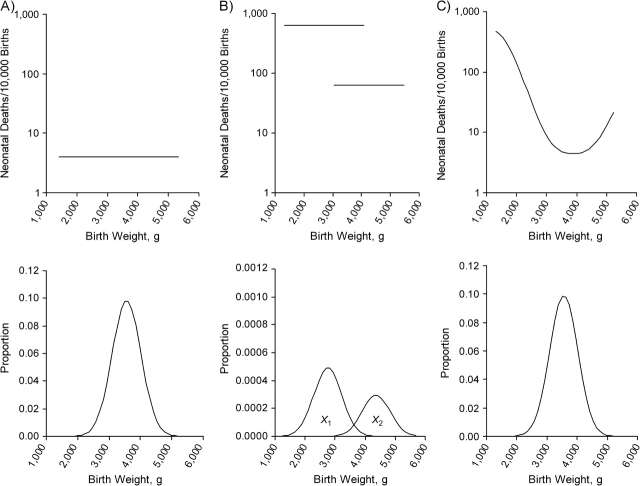
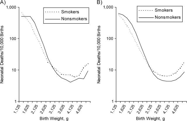
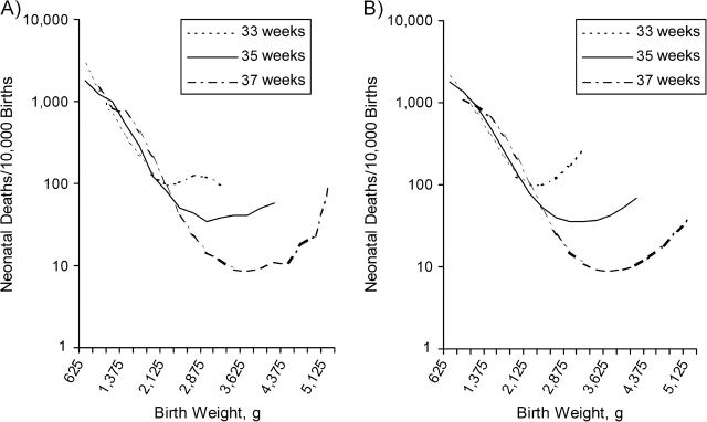
Small babies from a population with higher infant mortality often have better survival than small babies from a lower-risk population. This phenomenon can in principle be explained entirely by the presence of unmeasured confounding factors that increase mortality and decrease birth weight. Using a previously developed model for birth weight-specific mortality, the authors demonstrate specifically how strong unmeasured confounders can cause mortality curves stratified by known risk factors to intersect. In this model, the addition of a simple exposure (one that reduces birth weight and independently increases mortality) will produce the familiar reversal of risk among small babies. Furthermore, the model explicitly shows how the mix of high- and low-risk babies within a given stratum of birth weight produces lower mortality for high-risk babies at low birth weights. If unmeasured confounders are, in fact, responsible for the intersection of weight-specific mortality curves, then they must also (by virtue of being confounders) contribute to the strength of the observed gradient of mortality by birth weight. It follows that the true gradient of mortality with birth weight would be weaker than what is observed, if indeed there is any true gradient at all.

Figure 1.

Recapitulation of model's assumption. In A, a population has a mean birth weight of 3,500 g (standard deviation = 460) and mortality of 4 per 10,000 births. In B, 2 conditions, X₁ and X₂, affect 0.5% and 0.3%, respectively, of babies. Mortality is increased with odds ratios of 171 and 16, respectively, in babies with X₁ and X₂. (Note the different proportion scale in the y-axis of the birth weight distribution.) In C, the resulting mortality curve is shown.

Figure 2.

A population of babies exposed to factor F (broken line) is added to the previous scenario. In A, the population with factor F has a mean birth weight of 3,270 g (standard deviation = 460) and mortality 1.5 times that of babies without F. In B, X₁ and X₂ affect 0.5% and 0.3%, respectively, of babies in each population. The birth weight of babies with F is shifted to the left in these populations, as in the main distribution. The effect of X₁ and X₂ on the mortality of babies with F is increased with odds ratios of 171 and 16, respectively. (Note the different proportion scale in the y-axis of the birth weight distribution.) In C, the intersecting mortality curves in babies with and without F are shown.

Figure 3.

Figure 2C is enlarged to show the proportions of X₁ and X₂ in babies with and without factor F (refer to the text) in the stratum 2,200–2,300 g (enclosed in the box). The solid curve represents the birth weight distribution of babies without factor F; the broken curve represents the distribution of babies with factor F. Data are from Table 1.

Figure 4.

Empirical (A) and calculated (B) weight-specific mortality curves are shown for smokers and nonsmokers, an example with births between 38 and 42 weeks of gestation, estimated by the date of the last menstrual period. Simulation parameters are shown in Table 2. Empirical data are based on National Center for Health Statistics data, US livebirths, 1995–2002.

Figure 5.

Empirical (A) and calculated (B) weight-specific mortality curves are shown for births at 33, 35, and 37 weeks of gestation; weeks 33 and 35 are based on clinical estimates of gestation, while week 37 is based on the date of the last menstrual period. Simulation parameters are shown in Table 2. Empirical data are based on National Center for Health Statistics data, US livebirths, 1995–2002.

References

-
- Basso O, Wilcox AJ, Weinberg CR. Birth weight and mortality: causality or confounding? Am J Epidemiol. 2006;164(4):303–311. - PubMed
- Wilcox AJ. Birth weight and perinatal mortality: the effect of maternal smoking. Am J Epidemiol. 1993;137(10):1098–1104. - PubMed
- Hernandez-Diaz S, Schisterman EF, Hernan MA. The birth weight “paradox” uncovered? Am J Epidemiol. 2006;164(11):1115–1120. - PubMed
- Haig D. Meditations on birth weight: is it better to reduce the variance or increase the mean? Epidemiology. 2003;14(4):490–492. - PubMed
- Wilcox AJ. On the importance—and the unimportance—of birthweight. Int J Epidemiol. 2001;30(6):1233–1241. - PubMed
Publication types
MeSH terms
Grants and funding
LinkOut - more resources
Full Text Sources