The sparseness of neuronal responses in ferret primary visual cortex

Abstract

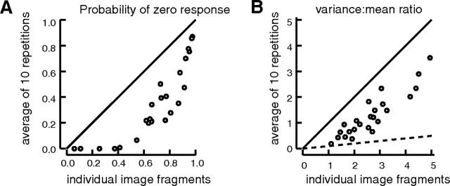
Various arguments suggest that neuronal coding of natural sensory stimuli should be sparse (i.e., individual neurons should respond rarely but should respond reliably). We examined sparseness of visual cortical neurons in anesthetized ferret to flashed natural scenes. Response behavior differed widely between neurons. The median firing rate of 4.1 impulses per second was slightly higher than predicted from consideration of metabolic load. Thirteen percent of neurons (12 of 89) responded to <5% of the images, but one-half responded to >25% of images. Multivariate analysis of the range of sparseness values showed that 67% of the variance was accounted for by differing response patterns to moving gratings. Repeat presentation of images showed that response variance for natural images exaggerated sparseness measures; variance was scaled with mean response, but with a lower Fano factor than for the responses to moving gratings. This response variability and the "soft" sparse responses (Rehn and Sommer, 2007) raise the question of what constitutes a reliable neuronal response and imply parallel signaling by multiple neurons. We investigated whether the temporal structure of responses might be reliable enough to give additional information about natural scenes. Poststimulus time histogram shape was similar for "strong" and "weak" stimuli, with no systematic change in first-spike latency with stimulus strength. The variance of first-spike latency for repeat presentations of the same image was greater than the latency variance between images. In general, responses to flashed natural scenes do not seem compatible with a sparse encoding in which neurons fire rarely but reliably.

Figure 1.

A, A schematic illustration of the protocol for presenting 150 × 150 pixel fragments of photographs of natural scenes. Each fragment was turned on suddenly for 100 ms and then removed suddenly; between fragments, the display CRT was held at a uniform midgray for 100–170 ms. B–E, Poststimulus time histograms for four neurons, showing the most likely times of action potential generation with respect to the presentation time of the natural scene fragments. The histograms are averaged across all the image fragments presented to each neuron.

Figure 2.

A, The histogram shows the latency of response of 86 neurons to the onset of the flashed natural scene stimuli. Latency is estimated from the PSTH averaged across all stimuli (like those in Fig. 1). This includes the latency of the small ON response for most of the neurons in which we have analyzed the sparseness of their larger OFF responses. Three neurons of the 89 are not included because either they gave only OFF responses or their responses were so weak that a clear “turn-up” in the PSTH at response onset was difficult to discern. B, The latency of the offset response for those 52 neurons with a clearly defined offset response. C, The latency of the offset response is plotted against the latency of the onset response. The symbols on the axes show the many cases (x-axis) in which a clear offset response was not discernible and a single case (y-axis) in which no onset response was obvious.

Figure 3.

Sparseness measures for eight hypothetical response distributions. A, A Gaussian distribution with mean response of zero should have kurtosis and entropy of zero, by definition. B, The same distribution as in A, but with all negative values set to zero; such “half-wave rectification” is a stylized model of the responses of simple cells with no spontaneous activity. C, The same distribution as in A, but with all negative values made positive and reflected through zero; such “full-wave rectification” is a stylized model of the responses of complex cells with no spontaneous activity. D, A stylized model of the response distribution of a simple cell with spontaneous level of activity equivalent to a response of “5 units”: 5 is added to the Gaussian distribution of A and all negative values are then set to zero. E, A leptokurtic distribution (exponential) with the same mean (zero) and variance as in A. F, G, Half-wave rectified and full-wave rectified versions of the exponential distribution in E. H, A stylized model of the responses of a simple cell with no spontaneous activity and with a response threshold equivalent to a response of “5 units”: 5 is subtracted from the Gaussian distribution of A, and all negative values are then set to zero.

Figure 4.

The numbers of action potentials generated by three neurons during 100 ms counting periods for 100 image fragments; these are part of the records of experiments in which 500 fragments were presented 10 times each to each neuron. The abscissas give an arbitrary i.d. code for which of the image fragments was presented (the responses to different fragments are shown for the 3 neurons). The ordinate shows the 10 repetitions of each stimulus. The square symbols show the number of action potentials generated in 100 ms for each repetition of each fragment; the area of the square is proportional to the number of action potentials evoked in the illustrated sequences (maximum responses: A, 9; B, 12; C, 12). The neuron of C had substantial spontaneous activity, and, to avoid clutter, only the responses to odd-numbered image fragments are shown.

Figure 5.

A–D, The distribution of response magnitudes for experiments on four neurons. A–C are the distributions for the three neurons whose rasters are shown in Figure 4A–C, respectively. The histograms show the proportion of image presentations of the total 5000 in which a particular action potential count was obtained. No account is taken at this stage that the 5000 presentations may have consisted of 10 repetitions of only 500 different images. The arrows point to largest response evoked for any one image presentation (9, 16, 17, and 44); the ordinate scales are such that the histogram bins for the most infrequent response magnitudes are difficult to discern from the abscissa lines. Four sparseness measures are shown for each histogram. For histograms A, B, and D, the full height of the bin is not shown at a response magnitude of zero; the proportion of zero responses is given by the P₀ sparseness metric. E, F, Distribution of the averaged response magnitudes for neurons A and B after the responses to the 10 repetitions of each image fragment are averaged together. Note the magnified x and y scales compared with histograms A and B. Note also that averaged responses are no longer integers but can be binned in steps of 0.1. The change in bin size has large effects on the calculation of distribution entropy.

Figure 6.

For the 89 neurons under study, the graphs in A–C plot the Treves–Rolls sparseness measure (TR) (A), kurtosis (k₄) (B), and entropy (S_E) (C) against the probability of obtaining a zero response (P₀). The gross outlier in C with entropy >3.0 is for the response distribution shown in Figure 5D. The correlation coefficients for these plots are given in Table 1. D, A histogram to show how many neurons were found with each level of sparseness; the filled blocks are for neurons with spontaneous activity >3 i.p.s.

Figure 7.

Plots to show the associations between the sparseness of response to natural image stimuli and other response properties. A, Relative modulation in the responses to moving sinusoidal gratings of optimal orientation and spatial frequency. B, Spontaneous activity. C, The bandwidth of the orientation tuning curve measured with moving sinusoidal gratings of optimal spatial frequency (see Baker et al., 1998). D, The bandwidth of the spatial-frequency tuning curve measured with moving sinusoidal gratings of optimal orientation. Bandwidths were measured as full width at half-amplitude. The correlation coefficients for these plots are given in Table 2. Filled symbols, Relative modulation, <1.0; open symbols, relative modulation, >1.0, the arbitrary dividing line by which some separate complex cells from simple cells (Skottun et al., 1991).

Figure 8.

Schematics to how the potential effects of response variability on the forms of simple cell response distributions for natural image stimuli. A and B show “clean” thresholded Gaussian distributions (replotted from Fig. 3B,H, respectively). Each of these occurrences is considered to be the mean value in a Poisson-like distribution, the underlying noise-free response to an image. Each occurrence in A and B is replaced in C and D by noise-corrupted values: each “clean” occurrence is first replaced from a randomly chosen sample from a Poisson distribution with parameter equal to the “clean” response; then, that sample is in turn replaced with a randomly chosen sample from a second Poisson distribution with parameter equal to the interim “noisy” value. This gives variance approximately equal to twice the mean response level for any particular stimulus. Note that response noise increases the number of zero responses and also the length of the distribution tail at high response magnitudes.

Figure 9.

For 24 neurons, 500 image fragments were presented 10 times each. The graphs show the effects on the response distributions of averaging the responses to the 10 repetitions of each fragment. The abscissas show measures of the distributions of the 5000 individual responses; the ordinates show the equivalent measures of the distributions of the 500 averaged responses. The solid lines are the lines of equality. A, P₀, the probability of obtaining a zero response either to individual stimulus presentations (abscissa) or on average to particular image fragments (ordinate). B, The variance of the distribution of responses divided by the mean response. The overall variance of the distribution is lowered by averaging responses to stimulus repetitions, but the mean response is, of course, unchanged. The dashed line has a slope of 1/10 and shows how much the variance of the response distribution could have been reduced by averaging 10 repetitions, if the whole variety of responses to natural images was attributable to response variability.

Figure 10.

A, B, The variance of response to 10 repetitions of each natural image fragment is plotted against the mean response to that fragment for the two neurons illustrated in Figures 4, A and B, and 5, A and B, and E and F. Data with mean response of zero cannot be plotted on the log–log axes; there are fewer data plotted in A because the responses of this neuron were sparser than the responses of B (Figs. 4A,B, 5A,B). The lines are the lines of equality. Regression lines fitted to those points with abscissa value 0.4 and above had slope and intercept: 0.951, 1.238 (A), and 0.707, 0.783 (B). The intercept is the average ratio of variance to mean response for that neuron. C, For 24 neurons, the average variance/mean-response ratio was calculated for those flashed natural image stimuli giving a mean response of at least 0.4 action potentials per presentation and is plotted as ordinate against the variance/mean-response ratio for moving high contrast sinusoidal gratings. The ratio for natural image stimuli was calculated from 10 repetitions of up to 500 stimuli; the ratio for gratings was calculated for 30 cycles of up to 12 stimuli, varying in spatial frequency or orientation. The line is the line of equality.

Figure 11.

For three neurons (A–C, respectively), the figure shows three PSTHs summarizing the responses to three different image sets. Neuron B is the same as in Figure 1C; neuron C is the same as in Figure 1E. For each neuron, the 500 stimulus images were ranked according to the number of action potentials evoked over the whole stimulus interval including the blank between images. The top row of histograms shows PSTHs summed only across the 20 most powerful stimuli for each neuron; the middle rows sums the responses to stimuli ranked 41–70 for each neuron; whereas the bottom row sums the responses to stimuli ranked 101–150 for each neuron. The response bins are 4 ms. Note the expansion in the y-axis scale as one proceeds down the rows.

Figure 12.

The rasters show the times of action potentials of four neurons in response to repetitions of different subsets of the 500 images. For each neuron, the responses are shown for the 20 images that evoked the greatest response on average from the respective neuron and a further 20+ images that evoked weak responses. The rows of the rasters are grouped in 10 s (A, C, D) (or 11 s; B), the number of repeats, with gaps to separate the responses to the different images. The black and red symbols show the times of action potentials after stimulus onset (B–D) or offset (A); the red symbols show the first spike after the stimulus transition in each raster row. The green symbols show those stimulus presentations that elicited no action potentials at all.

References

1. Atick JJ, Redlich AN. What does the retina know about natural scenes? Neural Comput. 1992;4:196–210.
1. Attwell D, Laughlin SB. An energy budget for signaling in the grey matter of the brain. J Cereb Blood Flow Metab. 2001;21:1133–1145. - PubMed
1. Baddeley R, Abbott LF, Booth MC, Sengpiel F, Freeman T, Wakeman EA, Rolls ET. Responses of neurons in primary and inferior temporal visual cortices to natural scenes. Proc Biol Sci. 1997;264:1775–1783. - PMC - PubMed
1. Baker GE, Thompson ID, Krug K, Smyth D, Tolhurst DJ. Spatial frequency tuning and geniculocortical projections in the visual cortex (areas 17 and 18) of the pigmented ferret. Eur J Neurosci. 1998;10:2657–2668. - PubMed
1. Bardy C, Huang JY, Wang C, FitzGibbon T, Dreher B. “Simplification” of responses of complex cells in cat striate cortex: suppressive surrounds and “feedback” inactivation. J Physiol. 2006;574:731–750. - PMC - PubMed
Publication types
LinkOut - more resources