. 2009;4(3):e4638.
doi: 10.1371/journal.pone.0004638. Epub 2009 Mar 4.

Lip-reading aids word recognition most in moderate noise: a Bayesian explanation using high-dimensional feature space

Affiliations

Lip-reading aids word recognition most in moderate noise: a Bayesian explanation using high-dimensional feature space

Wei Ji Ma et al. PLoS One. 2009.

Abstract

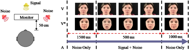
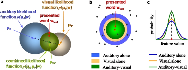
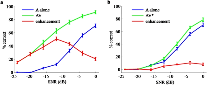
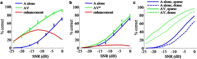
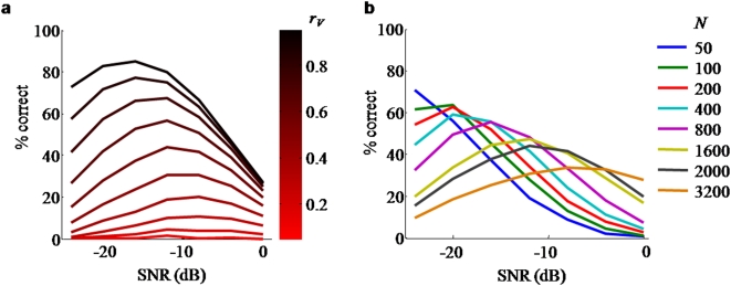
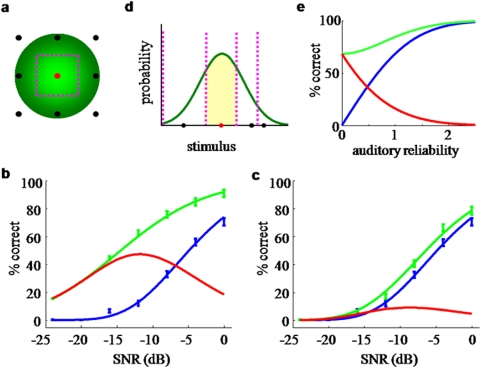
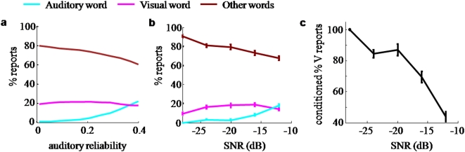
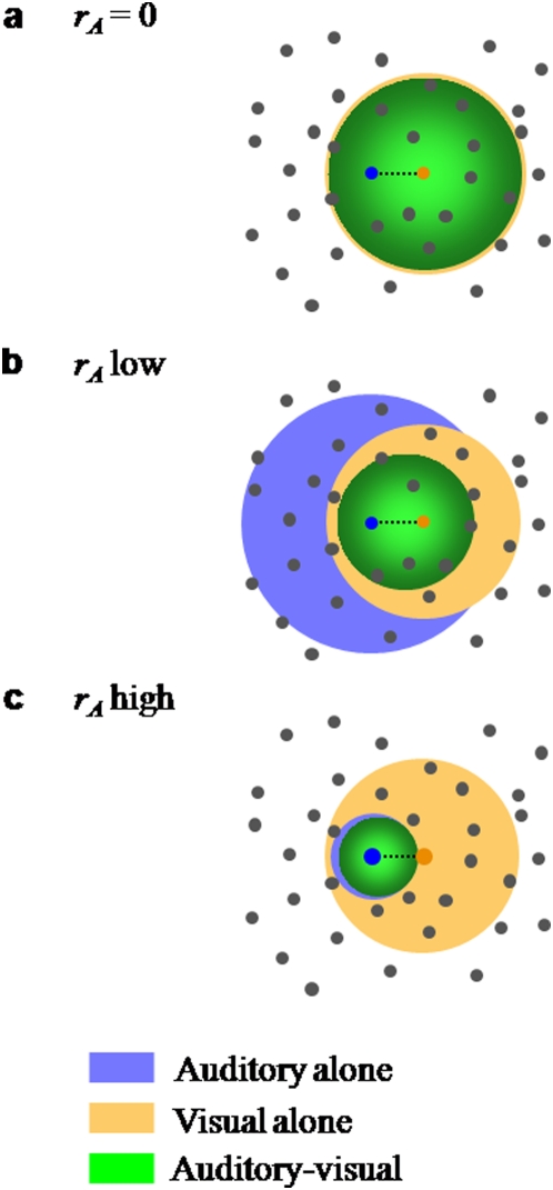
Watching a speaker's facial movements can dramatically enhance our ability to comprehend words, especially in noisy environments. From a general doctrine of combining information from different sensory modalities (the principle of inverse effectiveness), one would expect that the visual signals would be most effective at the highest levels of auditory noise. In contrast, we find, in accord with a recent paper, that visual information improves performance more at intermediate levels of auditory noise than at the highest levels, and we show that a novel visual stimulus containing only temporal information does the same. We present a Bayesian model of optimal cue integration that can explain these conflicts. In this model, words are regarded as points in a multidimensional space and word recognition is a probabilistic inference process. When the dimensionality of the feature space is low, the Bayesian model predicts inverse effectiveness; when the dimensionality is high, the enhancement is maximal at intermediate auditory noise levels. When the auditory and visual stimuli differ slightly in high noise, the model makes a counterintuitive prediction: as sound quality increases, the proportion of reported words corresponding to the visual stimulus should first increase and then decrease. We confirm this prediction in a behavioral experiment. We conclude that auditory-visual speech perception obeys the same notion of optimality previously observed only for simple multisensory stimuli.


Conflict of interest statement

Competing Interests: The authors have declared that no competing interests exist.

Figures

Figure 1
Figure 1. Experimental set-up and timing of audio-visual stimuli.
Figure 2
Figure 2. Bayesian model of auditory-visual word recognition.
a. Inference process on a single multisensory trial. Word prototypes are points in a high-dimensional space (of which two dimensions are shown). The presented word (in red) gives rise to an auditory (μA) and a visual (μV) observation (which are the respective unisensory estimates if only one modality is presented). Based on these, the brain constructs likelihood functions over utterances w, indicated by muted-colored discs. The diameter of a disc is proportional to the standard deviation of the Gaussian. The auditory-visual likelihood is the product of the unisensory likelihoods and is centered at μAV (see text), which is the multisensory estimate on this trial. b. Across many repetitions of the test word, the estimates will form a distribution centered at the test word. The estimate distributions are shown as bright-colored discs for the auditory-alone (A), visual-alone (V), and auditory-visual (AV) conditions. Since the distributions “cover” many words, errors will be made. Note the different interpretations of the discs in a and b: single-trial likelihood functions, versus estimate distributions across many trials. c. Side view of the estimate distributions in b. The AV estimate distribution is sharper than both the A and the V distribution, leading to fewer errors. This indicates the advantage conferred by multisensory integration.
Figure 3
Figure 3. Behavioral performance in open-set word recognition.
Data consisted of auditory-alone performance (blue) and auditory-visual performance (green). The multisensory enhancement (red) is the difference between auditory-visual and auditory-alone performance. Error bars indicate s.e.m. a: Full visual information (AV). b: Impoverished visual information (AV*). In both cases, maximum enhancement occurs at intermediate values of auditory SNR.
Figure 4
Figure 4. A Bayesian model of speech perception can describe human identification performance.
A vocabulary of size N = 2000 was used. Words were distributed in an irregular manner in a space of dimension n = 40. For details of the fits, see the Supplemental Material. a: Data (symbols) and model fits (lines) for A-alone and AV conditions. The red line is the multisensory enhancement obtained from the model. b: Same for impoverished visual information (AV*). c: Words in high-density regions are harder to recognize. In the simulation in a, words were categorized according to their mean distance to other words. When the mean distance is large (sparse, solid lines), recognition performance in both A-alone and AV conditions is higher than when the mean distance is small (dense, dashed lines).
Figure 5
Figure 5. Predictions of the Bayesian model for auditory-visual enhancement as a function of auditory SNR, for various values of:
a: visual reliability (from 0.05 to 0.95 in steps of 0.10); b: vocabulary size. For both plots, all other parameters were taken from the fit in Figure 4. See Results for interpretation.
Figure 6
Figure 6. Optimal cue combination in multiple dimensions according to a simple analytical model.
a. In this simplified model, word prototypes (dots) lie on a rectangular grid, here shown in two dimensions. The green blob indicates an example estimate distribution (compare Fig. 2b). The dashed lines enclose the correctness region when the central word is presented. b and c. The model was fitted to the data in the AV condition (b) and the AV* condition (c). Data are shown as symbols, lines are model fits. Colors are as in Fig. 3. d. The same model in 1 dimension, but now allowing word prototypes to be unequally spaced. The green curve is an estimate distribution. The vertical dashed lines are the boundaries of the decision regions. The shaded area corresponds to correct responses when the presented stimulus is the one marked in red. e. Typical identification performance in 1 dimension, for the A (blue) and AV (green) conditions. The multisensory enhancement (red) decreases monotonically with auditory reliability. This is an instance of inverse effectiveness. For details, see the Supporting Information.
Figure 7
Figure 7. Effect of an auditory word on reports of an incongruent visual word.
a. Illustration of the Bayesian prediction. An experiment was simulated in which pairs of slightly incongruent auditory and visual words are presented. On each trial, the observer integrates the signals and reports a single word. Frequencies of reporting the auditory word (cyan), the visual word (magenta), and other words (brown) are shown as a function of auditory reliability. As auditory reliability increases, the percentage reports of the visual word reaches a maximum before it eventually decreases. This is a small but significant effect. Note that the interpretation of both curves is completely different from that of Figures 3–4 (here, the only condition is multisensory, and there is no notion of correctness). A vocabulary of size N = 2000 and dimension n = 30 were used, and visual reliability was fixed at rV = 0.5. Robustness of the effect across dimensions and vocabulary sizes is demonstrated in Figure S5. b. Experimental test of the Bayesian prediction. The percentage reports of the visual word exhibits a maximum as a function of SNR. The curves in a have not been fitted to those in b. c. Reports of the visual word as a percentage of the total reports of either the auditory or the visual word, computed from the data shown in b. As expected, this declines monotonically with SNR.
Figure 8
Figure 8. A large distracter set gets squashed.
This figure illustrates the Bayesian model for integrating slightly incongruent auditory-visual stimuli. Dots represent word prototypes. The blue and orange dots represent the auditory and visually presented words, respectively. Each disc represents a Gaussian maximum-likelihood estimate distribution (A, V, or AV); its radius is proportional to the standard deviation of the Gaussian. a–c differ in auditory reliability but not in visual reliability. In a, auditory reliability is zero, therefore the V and AV distributions are identical. As auditory reliability increases, the AV distribution sharpens (thereby excluding more and more distractors) and shifts more towards the auditory word. These two effects together initially benefit both the auditory and the visual word, since the visual word is close to the auditory word and enjoys some of the increased probability mass (compare a and b). Eventually, the benefit will go more exclusively to the auditory word (compare b and c). This explains why in Figure 7b the percentage of reports of the visual word in the AV condition first increases and then ultimately decreases. Note that the auditory and the visual word do not have to be nearest neighbors.

References

    1. Campbell R. Speechreading: advances in understanding its cortical bases and implications for deafness and speech rehabilitation. Scand Audiol. 1998;Suppl 49 - PubMed
    1. Bernstein LE, Demorest ME, Tucker PE. Speech perception without hearing. Perception and Psychophysics. Perception and Psychophysics. 2000;62:233–252. - PubMed
    1. Grant KW, Walden BE. Evaluating the articulation index for auditory-visual consonant recognition. J Acoust Soc Am. 1996;100:2415–2424. - PubMed
    1. MacLeod A, Summerfield Q. Quantifying the contribution of vision to speech perception in noise. Br J Audiol. 1987;21:131–141. - PubMed
    1. Massaro DW. Speech perception by ear and eye: A paradigm for psychological inquiry. Hillsdale, , NJ: Erlbaum; 1987.