Case Reports
. 2008:106:426-58.

Spectral domain optical coherence tomography for glaucoma (an AOS thesis)

Affiliations
Case Reports

Spectral domain optical coherence tomography for glaucoma (an AOS thesis)

Joel S Schuman. Trans Am Ophthalmol Soc. 2008.

Abstract

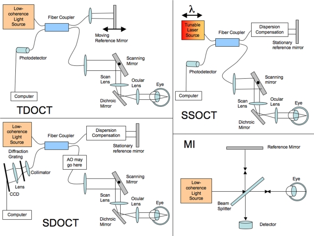
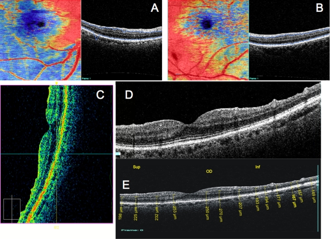
Purpose: Optical coherence tomography (OCT) is a rapidly evolving, robust technology that has profoundly changed the practice of ophthalmology. Spectral domain OCT (SD-OCT) increases axial resolution 2- to 3-fold and scan speed 60- to 110-fold vs time domain OCT (TD-OCT). SD-OCT enables novel scanning, denser sampling, and 3-dimensional imaging. This thesis tests my hypothesis that SD-OCT improves reproducibility, sensitivity, and specificity for glaucoma detection.

Methods: OCT progress is reviewed from invention onward, and future development is discussed. To test the hypothesis, TD-OCT and SD-OCT reproducibility and glaucoma discrimination are evaluated. Forty-one eyes of 21 subjects (SD-OCT) and 21 eyes of 21 subjects (TD-OCT) are studied to test retinal nerve fiber layer (RNFL) thickness measurement reproducibility. Forty eyes of 20 subjects (SD-OCT) and 21 eyes of 21 subjects (TD-OCT) are investigated to test macular parameter reproducibility. For both TD-OCT and SD-OCT, 83 eyes of 83 subjects are assessed to evaluate RNFL thickness and 74 eyes of 74 subjects to evaluate macular glaucoma discrimination.

Results: Compared to conventional TD-OCT, SD-OCT had statistically significantly better reproducibility in most sectoral macular thickness and peripapillary RNFL sectoral measurements. There was no statistically significant difference in overall mean macular or RNFL reproducibility, or between TD-OCT and SD-OCT glaucoma discrimination. Surprisingly, TD-OCT macular RNFL thickness showed glaucoma discrimination superior to SD-OCT.

Conclusions: At its current development state, SD-OCT shows better reproducibility than TD-OCT, but glaucoma discrimination is similar for TD-OCT and SD-OCT. Technological improvements are likely to enhance SD-OCT reproducibility, sensitivity, specificity, and utility, but these will require additional development.
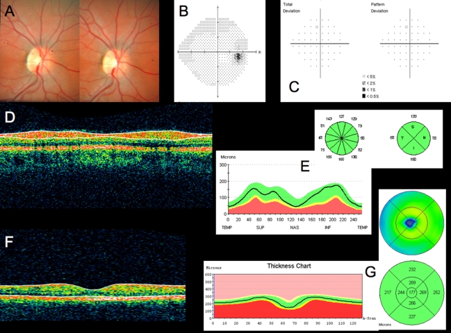
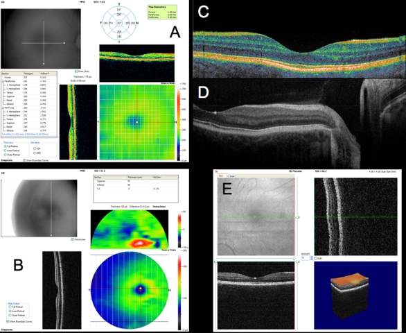
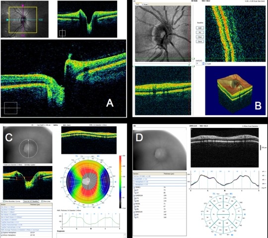
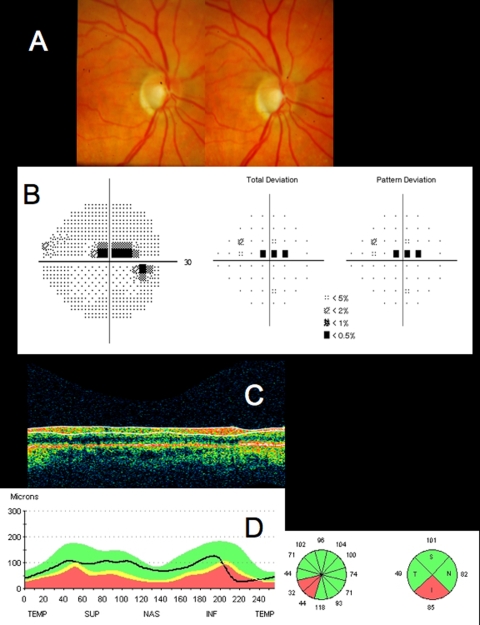

Figures

FIGURE 1
FIGURE 1
Optical coherence tomography (OCT) schematics: time-domain OCT (TD-OCT), spectral-domain OCT (SD-OCT), swept-source OCT (SS-OCT), and the adaptive optics system that can be added into a SD-OCT system (AO-OCT). Light signals are split and exchanged through the fiber coupler. The scanning mirror scans the beam across to make a B-scan. The dispersion correction of SD-OCT and SS-OCT corrects for light dispersion through the length of the eye and can be done through software after acquisition or through a material like a cuvette of distilled water approximately the length of the eye to compensate. The collimator in SD-OCT collects the light to shine it through a diffraction grating that spreads the different frequencies of light across the charge-coupled device (CCD) camera.
FIGURE 2
FIGURE 2
Spectral domain optical coherence tomography with adaptive optics schematics: The adaptive optics portion of the system is in the dotted box. The wavefront sensor in the adaptive optics system detects the aberrations occurring in the light and sends this information in a feedback loop to the deformable mirror (connection not shown).
FIGURE 3
FIGURE 3
Spectral domain optical coherence tomography B-scan from macula to optic disc, with retinal layers labeled: RNFL, retinal nerve fiber layer; GCL, ganglion cell layer; IPL, inner plexiform layer; INL, inner nuclear layer; OPL, outer plexiform layer; ONL, outer nuclear layer; ELM, external limiting membrane; IS/OS PhR, boundary between inner and outer segments of the photoreceptors; RPE, retinal pigment epithelium.
FIGURE 4
FIGURE 4
Areas of macular thickness segmentation: C, center; OS, outer superior; ON, outer nasal; OI, outer inferior; OT, outer temporal; IS, inner superior; IN, inner nasal; II, inner inferior; IT, inner temporal. Weighted mean is taken across the entire circle.
FIGURE 5
FIGURE 5
Conventional testing images from healthy case study: A, Stereoscopic disc photographs of a 23-year-old white woman’s healthy right eye. B, Humphrey SITA 24–2 threshold map of healthy right eye. C, Total deviation and pattern deviation maps showing no significant deviation from normative values. D, Time domain ocular coherence tomography (TD-OCT) retinal nerve fiber layer (RNFL) thickness OCT scan, with white lines delineating RNFL boundaries. The white lines are automatically placed by software that automatically identifies the tissue borders of interest, but should always be checked by the clinician for accuracy. E, RNFL segmentation results superimposed on normative database. Green is within normal limits (5th to 95th percentile), yellow is borderline (1st to 4th percentile) and red is outside normal limits (below the 1st percentile). Wheels present quadrant and clock hour averaged thicknesses. All green results indicate RNFL thickness is within normal limits. F, TD-OCT macular thickness OCT scan, with white lines designating total retinal thickness segmentation results. G, Single macular scan and macular map results. Single scan and overall measured thicknesses are compared to normative values. Map represents thicker measurements with warmer colors, and thinner measurements with cooler colors (eg, the fovea is dark blue, as the thinnest region in the healthy eye).
FIGURE 6
FIGURE 6
Macular spectral domain optical coherence tomography (SD-OCT) images from healthy case study shown in Figure 5. A, RTVue MM5 output, with fundus camera view, vertical and horizontal OCT scans through macula, macular map, and tabular thickness measurements. B, RTVue MM7 output, with macular map, map of superior-inferior thickness differences, and vertical OCT B-scan through the macula. The red area indicating a large difference between the superior and inferior hemispheres at that point is an artifact of slight decentration of the macula vertically in that scan. C, High-resolution color mapped SD-OCT line scan through macula acquired by research device created at Massachusetts Institute of Technology, displaying retinal layers clearly. D, High-resolution grayscale SD-OCT line scan through macula and optic nerve head acquired by Bioptigen SD-OCT device. E, Macular 3D data set acquired by RTVue SD-OCT. Upper left is the OCT fundus image. Lower left and upper right B-scans are at the locations of the green and red lines on the OCT fundus image, respectively. 3D representation is at lower right.
FIGURE 7
FIGURE 7
Optic nerve head (ONH) and retinal nerve fiber layer (RNFL) spectral domain optical coherence tomography (SD-OCT) images from healthy case study shown in Figures 5 and 6: A, Cirrus HD-OCT ONH 3D data set. Lower B-scan and upper B-scans are from position of blue and purple lines on the fundus view, respectively. B, RTVue ONH 3D data set. Upper left is en face image. Note vessel disconnect near top, indicating eye motion. Lower left and upper right B-scans are at the locations of the green and red lines on the en face image, respectively. 3D representation is at lower right. C, RTVue NHM4 scan pattern output. NHM4 is a pattern of radial scans combined with circular scans. Fundus view is in upper left. Radial B-scan and circular B-scan are indicated by red; white lines imposed over the RNFL thickness map represent other acquired scans. Warm colors in the map represent thick, healthy nerve fiber bundles. The 3.4-mm-diameter circle thickness graph and other parameter measurements are presented. D, RTVue RNFL scan pattern output. RNFL scan consists of four 3.4-mm-diameter circles around the ONH, whose RNFL segmentation thickness measurements are averaged. Sectorally averaged thicknesses are displayed in the round chart.
FIGURE 8
FIGURE 8
Standard clinical images from a patient with early glaucoma and a focal retinal nerve fiber layer (RNFL) defect. A, Stereoscopic disc photographs of right eye with inferotemporal defect, visible as marked cupping. B, Humphrey SITA 24–2 visual field threshold, total deviation, and pattern deviation maps, with superior paracentral scotoma. C, Time domain optical coherence tomography (TD-OCT) RNFL OCT scan. D, Comparison of TD-OCT RNFL thickness to normative database, with the inferior temporal RNFL thickness outside normal limits (red), consistent with visual field loss and optic nerve head loss of neuroretinal rim.
FIGURE 9
FIGURE 9
Spectral domain optical coherence tomography (SD-OCT) scans from the patient shown in Figure 8 with early glaucoma and a focal retinal nerve fiber layer (RNFL) defect. A, RTVue RNFL scan output. Note the clear inferior temporal notch, which can be more clearly measured without the oversmoothing problem of time domain OCT. B, RTVue 3D optical nerve head (ONH) 3D data set. Note how the tissue loss can be clearly seen in the B-scan obtained at the green line on the en face image, visible in the lower left corner. C, RTVue NHM4 scan output. Black and dark blue area inferior temporally indicates area of focal loss. The rest of the scan appears fairly healthy and thick. D, RTVue 3D data set from a macular scan, with 3D representation.
FIGURE 10
FIGURE 10
Standard clinical images from a patient with advanced glaucoma and global retinal nerve fiber layer (RNFL) and visual loss: A, Stereoscopic disc photograph showing overall neuroretinal rim loss in the optic disc, evidenced by marked optic nerve cupping. B, Humphrey SITA 24–2 visual field threshold, total deviation, and pattern deviation maps, with central inferior scotoma and temporal superior loss. C, Time domain optical coherence tomography RNFL scan, with RNFL thickness segmentation. Note slight segmentation error due to algorithm oversmoothing of the anterior RNFL tissue border superiorly. D, Comparison of RNFL thickness to normative database. RNFL loss results in nearly all areas showing thicknesses that are borderline or outside normal limits, except the nasal portion, where tissue loss typically appears last. The RNFL is markedly thin superiorly and inferiorly.
FIGURE 11
FIGURE 11
Spectral domain optical coherence tomography (SD-OCT) scans from the patient shown in Figure 10 with advanced glaucoma and global retinal nerve fiber layer (RNFL) and visual loss. A, RTVue RNFL scan output. Note the improved segmentation superiorly, compared to time-domain OCT (TD-OCT) in Figure 10C. B, RTVue optical nerve head (ONH) 3D data set, showing larger area of optic nerve cupping and thin neuroretinal rim. C, RTVue MM5 macular scan output, showing temporal thinning with advanced glaucoma. D, RTVue MM7 macular scan output, also showing temporal loss, and overall thinning. This figure shows inner retinal thickness specifically, using a relatively new segmentation algorithm that allows segmentation of the intraretinal layers beyond simply total retinal thickness and macular RNFL thickness. This algorithm also permits superior to inferior macular comparison by subtraction, as shown in the upper panel of Figure 11D. This demonstrates asymmetry in inner retinal thickness, with the inner retina thinner inferiorly than superiorly, consistent with the RNFL thickness shown in Figures 10 C and D and 11A and the visual field shown in Figure 10B. Note on the visual field (Figure 10B) that while there is perimetric damage both above and below the horizontal meridian, with a superior nasal defect and an inferior paracentral scotoma, the inferior defect is considerably deeper than the superior one, as borne out by the TD-OCT and SD-OCT. E, RTVue NHM4 scan output shows extensive RNFL thinning, with minimal areas represented with warm colors, and substantial black and dark blue areas.
FIGURE 12
FIGURE 12
Standard clinical images from a patient with glaucoma progression. Two visits were a year apart: ’06 denotes image from first visit, ’07 denotes image from second visit. A, Disk photograph from second visit. Disc or fundus photography was not obtained at the first visit. B, Humphrey SITA 24–2 visual field threshold maps from first and second visit. C, Glaucoma progression analysis output between the two visits. Some inferior-temporal points were already too depressed to show progression, but significant progression occurred around the scotoma demonstrated at the first visit. D, Total and pattern deviation maps. These show similar progression to the other visual field analyses.
FIGURE 13
FIGURE 13
Optical coherence tomography (OCT) images from the patient in Figure 12 with glaucoma progression: Two visits were a year apart: ’06 denotes image from first visit, ’07 denotes image from second visit. A, Time-domain OCT retinal nerve fiber layer (RNFL) thicknesses compared to the normative database. Possible progression is shown inferiorly, but it is difficult to determine if appearance of progression is due to changes in 3.4-mm circle centration between scans. B, RTVue MM7 scans show overall macular scanning, with the superior hemisphere losing more tissue, bringing it more similar to the lower thickness of the inferior hemisphere. C, RTVue RNFL scans can be compared on its software to clearly show progression. RNFL thickness loss can be seen over nearly the entire circle, except inferior nasally. D, RTVue NHM4 RNFL thickness maps show loss overall, especially inferior temporally. E, RTVue optical nerve head (ONH) 3D data sets as 3D visualization also show increased cupping and RNFL tissue loss.
FIGURE 14
FIGURE 14
Standard clinical images from a patient with possible glaucoma: differential diagnosis case. A, Optic disc photograph from right eye. B, Optomap (Optos, Dunfemline, Scotland) fundus photograph showing peripheral retinal damage due to prior retinal detachment. Scarring is present around the closed retinal hole in the temporal periphery. C, Humphrey SITA 24–2 visual field threshold map showing superior temporal scotoma. D, Time domain optical coherence tomography (TD-OCT) RNFL imaging with segmentation. E, TD-OCT macular scan, showing a thin retina, but impossible to identify layers in which damage occurred. E, TD-OCT RNFL thickness comparison to normative database. Thinning is evident inferiorly, but depth location of thinning is not obvious.
FIGURE 15
FIGURE 15
Spectral comain optical coherence tomography (SD-OCT) images from the patient in Figure 14 with possible glaucoma: differential diagnosis case: A and B, Total retinal thickness segmentation software of our own design on macular 3D data sets from the right eye and left eye, respectively. Macula is in the top half of each image. Retinal thickness loss is evident inferior to the macula in the right eye compared to the left eye (blue is thinner than red), but it is unknown in which layer this loss occurred without examining the SD-OCT B-scans. C, Vertical scan from a SD-OCT 3D data set taken with the macula in the superior half of the scan. Note the tissue loss is in the inner retina, including the retinal nerve fiber layer (RNFL), retinal ganglion cell layer, and inner plexiform layer, with outer retinal layers measuring and appearing no different between the patient’s affected and unaffected eyes. D, Vertical OCT scan obtained by the Cirrus SD-OCT (left is the superior part of the scan, right is the inferior part of the scan). Retinal nerve fiber layer loss can be seen even more clearly in this scan, because of the device’s higher axial resolution and transverse scan density compared to time domain OCT, where the disease has left the retina with an irregular-appearing surface. E, Same scan as D, with aspect ratio of 1:1 to allow manual calipers retinal layer thickness measurements to assess which cellular layers of the retina are damaged.

References

    1. de Boer JF, Cense B, Park BH, Pierce MC, Tearney GJ, Bouma BE. Improved signal-to-noise ratio in spectral-domain compared with time-domain optical coherence tomography. Opt Lett. 2003;28:2067–2069. - PubMed
    1. Drexler W, Morgner U, Ghanta RK, Kartner FX, Schuman JS, Fujimoto JG. Ultrahigh-resolution ophthalmic optical coherence tomography. Nat Med. 2001;7:502–507. - PMC - PubMed
    1. Drexler W, Sattmann H, Hermann B, et al. Enhanced visualization of macular pathology with the use of ultrahigh-resolution optical coherence tomography. Arch Ophthalmol. 2003;121:695–706. - PubMed
    1. Fujimoto JG. Optical coherence tomography for ultrahigh resolution in vivo imaging. Nat Biotechnol. 2003;21:1361–1367. - PubMed
    1. Fujimoto JG, Pitris C, Boppart SA, Brezinski ME. Optical coherence tomography: an emerging technology for biomedical imaging and optical biopsy. Neoplasia. 2000;2:9–25. - PMC - PubMed

Publication types

MeSH terms