The importance of proving the null

Abstract

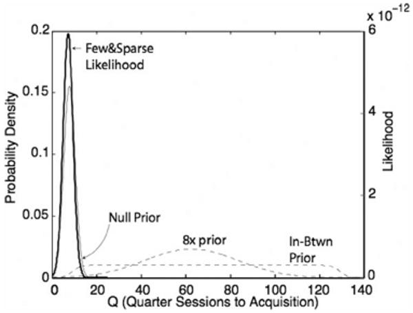
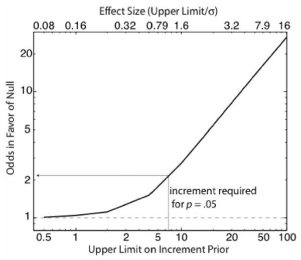
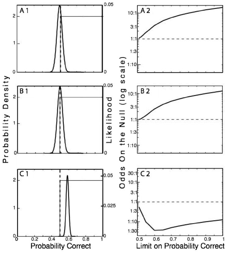
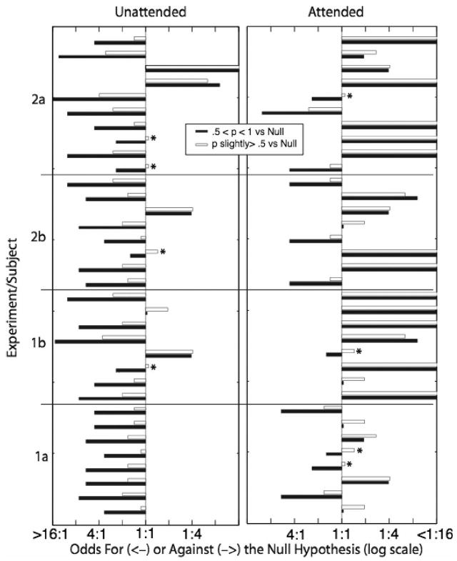
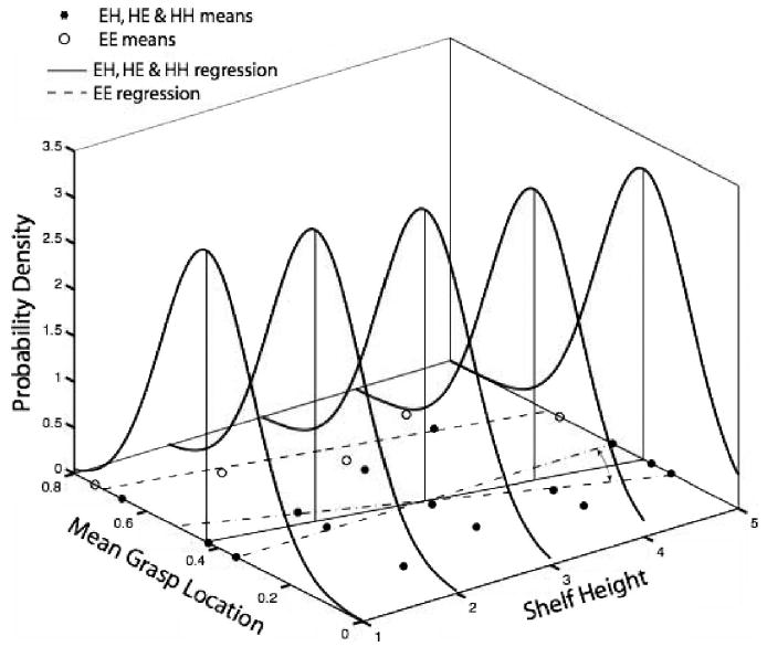
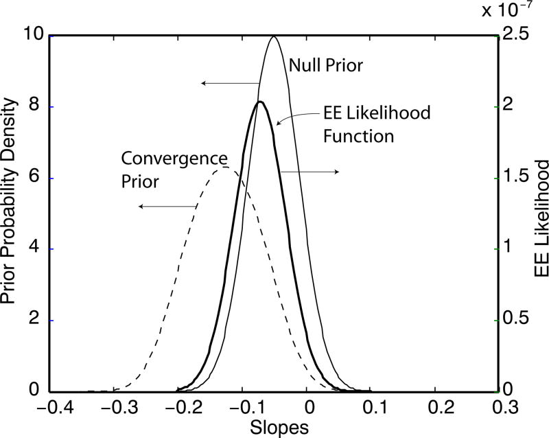
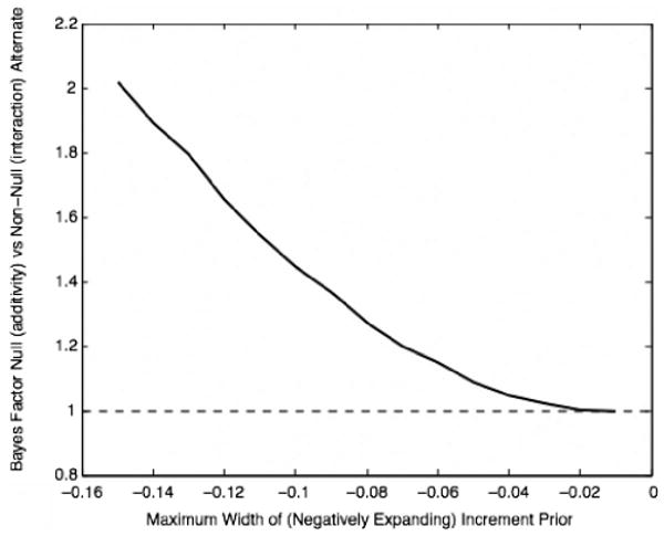
Null hypotheses are simple, precise, and theoretically important. Conventional statistical analysis cannot support them; Bayesian analysis can. The challenge in a Bayesian analysis is to formulate a suitably vague alternative, because the vaguer the alternative is (the more it spreads out the unit mass of prior probability), the more the null is favored. A general solution is a sensitivity analysis: Compute the odds for or against the null as a function of the limit(s) on the vagueness of the alternative. If the odds on the null approach 1 from above as the hypothesized maximum size of the possible effect approaches 0, then the data favor the null over any vaguer alternative to it. The simple computations and the intuitive graphic representation of the analysis are illustrated by the analysis of diverse examples from the current literature. They pose 3 common experimental questions: (a) Are 2 means the same? (b) Is performance at chance? (c) Are factors additive?

Figure 1

Schematic representation of (a portion of) two different classical conditioning protocols of equal duration but with an eightfold difference in the number of trials (CS-US pairings) in a given amount of time (t). Gottlieb (2008) tested the hypothesis that these two protocols have equivalent effects on the progress of learning.

Figure 2

The number of reinforced trials (CS-US pairings) to acquisition in a standard classical conditioning protocol with pigeon subjects, plotted against the ratio of the US-US and CS-US intervals, on double logarithmic coordinates. (Replotted from Gibbon & Balsam, 1981.) US-US is the average interval between USs (a.k.a. reinforcements). CS-US is the duration of the warning interval, commonly called the delay of reinforcement. As the (US-US)/(CS-US) ratio grows, this delay becomes relatively small, making it a relatively better predictor of imminent reinforcement. That is, the CS becomes more informative (Balsam & Gallistel, 2009). The slope of the regression (light solid line) does not differ significantly from −1 (heavy solid line). If it truly is −1 (itself a null hypothesis), then when trials are deleted, the increase in the informativeness of the CS precisely compensates for the decrease in the number of trials, in which case the number of trials is not itself important. What is important is the informativeness of the trials. t = time.

Figure 3

Cumulative distributions of quarter sessions to acquisition for two groups in Gottlieb's (2008) Experiment 4. These empirical cumulative distributions step up at the locus of each datum. Thus, the number of steps indicates the N (N_M&D = 6; N_F&S = 8), and the location along the Q axis of any one step is the Q for one subject. The dashed curve is a cumulative Gaussian with a standard deviation of 6.3, which is the pooled maximum unbiased estimate of the standard deviation of the distribution from which the data are drawn (assuming that the source distributions have a common variance, but not necessarily a common mean).

Figure 4

Computing a likelihood function. The assumed source distribution (the statistical model) is slid along the abscissa (here the μ axis), on which are plotted the known data (solid dots, labeled d₁–d₆ in middle panel, which are the data from the Many & Dense group). The top two panels show it at two locations. At each location, the likelihoods are read off (arrows projecting up from 3 of the 6 data points and over to the corresponding likelihoods). The product of the likelihoods is the likelihood of that location (that value of μ), given the data. The likelihood function (bottom panel) is the plot of the likelihood as a function of the possible locations of the source distribution, possible values of μ_Q. Note that the area under the likelihood function is nowhere near one (numbers on ordinate of bottom panel are × 10⁻⁹).

Figure 5

The likelihood function for the mean of the one-trial-per-quarter-session group (heavy curve) and the three prior probability functions corresponding to three different hypotheses: (a) the null hypothesis, which is that the quarter-sessions-to-acquisition data from this group were drawn from the same distribution as the data from the eight-trials/quarter sessions group; (b) the 8× hypothesis, which is that only trials matter, in which case the data from the one-trial group were drawn from a distribution eight times wider; (c) the vague hypothesis that the effect of reducing the number of trials per quarter session from eight to one has an effect somewhere within the range delimited by the null and the 8× hypotheses. The prior probability distributions are plotted against the left axis. They all, of course, integrate to one. The likelihood function is plotted against the right axis; it does not integrate to one.

Figure 6

The odds in favor of the null as a function of the assumed upper limit on the possible size of the effect (double logarithmic coordinates). The dashed line at 1 is where the odds ratio reverses (from favoring the null to favoring the vaguer alternative). Because the plot approaches this reversal point from above as the limit on vagueness goes to 0, the null is unbeatable by any alternative that posits some effect, no matter how small. The thin arrow shows the difference in the sample means that would be just significant at the .05 level. The odds are better than 2:1 against the hypothesis that the effect of deleting seven out of every eight trials is so small that it would be at most just detectable by a conventional null hypothesis significance test with samples this size.

Figure 7

Left: Likelihood functions (heavy curves, plotted against right axes) and competing prior probability functions (plotted against left axes) for chance (heavy vertical dashed lines at p = .5) and for greater than chance (light rectangles with height = 2, with left edge at .5 and right edge at 1). Right: Odds on the null as a function of the upper limit on the possible probability of a correct. A. Turk-Browne, Jungé, and Scholl's (2005) Experiment 1a, unattended color. B. Turk-Browne et al.'s Experiment 2a, unattended color. C. Turk-Browne et al.'s Experiment 1a, attended color.

Figure 8

Odds for (leftward projecting bars) or against (rightward projecting bars) the null hypothesis (chance), for each of 34 subjects in four experiments with tests of unattended and attended triplets. For each subject and each test, the null is pitted against two different alternatives: the probability of correct identification lies anywhere on the interval from .5 to 1 (black bars), or it lies between .5 and .65 (i.e., it is at most only slightly greater than chance). Asterisks mark instances in which the odds favor the null when pitted against the vaguer hypothesis but are against the null when it is pitted against the less vague alternative.

Figure 9

The heavy solid curves are copies of a common source distribution. Each copy is centered on the regression line, which, like all regression lines, is constrained to pass through the centroid of the data (at Level 3). The positions of the copies at Levels 1, 2, 4, and 5, relative to the underlying data (hence, also the likelihoods), depend on the slope of the regression line. The maximally likely regression lines for the base and easy-easy (EE) data are also plotted on the base plane, along with the data (solid line and dashed line). When we vary the slope of the regression line through the base data (curved arrows and dashed-dot lines) and compute the likelihood of the data as a function of that slope, we get the likelihood function for the slope. HE = hard-easy; HH = hard-hard.

Figure 10

The null prior and convergence prior for the slope of the regression line through Subject 7's easy-easy (EE) data (plotted against left axis), together with the likelihood function for the slope of those data (plotted against right axis).

Figure 11

The Bayes factor for the null versus convergence comparison as a function of the assumed upper limit on the rate of convergence (upper limit on how much more negative the easy-easy slope is than the base slope). The dashed line at 1 represents equal odds. The odds converge on this line. For any non-negligible width of the increment prior, the odds favor the null hypothesis (additivity).

References

1. Balsam P, Gallistel CR. Temporal maps and informativeness in associative learning. Trends in Neurosciences. 2009;32(2):73–78. - PMC - PubMed
1. Berger J, Moreno E, Pericchi L, Bayarri M, Bernardo J, Cano J, et al. An overview of robust Bayesian analysis. TEST. 1994;3(1):5–124.
1. Estes WK. The problem of inference from curves based on group data. Psychological Bulletin. 1956;53:134–140. - PubMed
1. Estes WK, Maddox WT. Risks of drawing inferences about cognitive processes from model fits to individual versus average performance. Psychonomic Bulletin & Review. 2005;12(3):403–409. - PubMed
1. Gallistel CR, Balsam PD, Fairhurst S. The learning curve: Implications of a quantitative analysis. Proceedings of the National Academy of Sciences of the United States of America. 2004;101(36):13124–13131. - PMC - PubMed