Gaussian-process factor analysis for low-dimensional single-trial analysis of neural population activity

Abstract

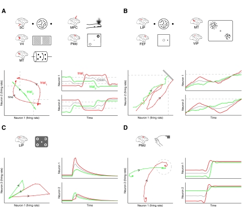
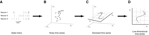
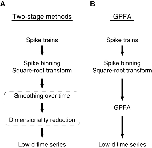
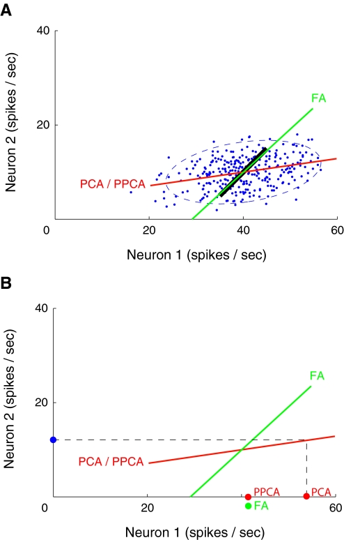
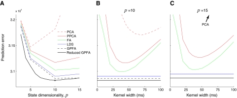
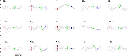
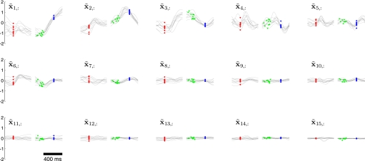
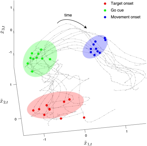
We consider the problem of extracting smooth, low-dimensional neural trajectories that summarize the activity recorded simultaneously from many neurons on individual experimental trials. Beyond the benefit of visualizing the high-dimensional, noisy spiking activity in a compact form, such trajectories can offer insight into the dynamics of the neural circuitry underlying the recorded activity. Current methods for extracting neural trajectories involve a two-stage process: the spike trains are first smoothed over time, then a static dimensionality-reduction technique is applied. We first describe extensions of the two-stage methods that allow the degree of smoothing to be chosen in a principled way and that account for spiking variability, which may vary both across neurons and across time. We then present a novel method for extracting neural trajectories-Gaussian-process factor analysis (GPFA)-which unifies the smoothing and dimensionality-reduction operations in a common probabilistic framework. We applied these methods to the activity of 61 neurons recorded simultaneously in macaque premotor and motor cortices during reach planning and execution. By adopting a goodness-of-fit metric that measures how well the activity of each neuron can be predicted by all other recorded neurons, we found that the proposed extensions improved the predictive ability of the two-stage methods. The predictive ability was further improved by going to GPFA. From the extracted trajectories, we directly observed a convergence in neural state during motor planning, an effect that was shown indirectly by previous studies. We then show how such methods can be a powerful tool for relating the spiking activity across a neural population to the subject's behavior on a single-trial basis. Finally, to assess how well the proposed methods characterize neural population activity when the underlying time course is known, we performed simulations that revealed that GPFA performed tens of percent better than the best two-stage method.

FIG. 1.

Conceptual illustration showing how the analytical methods presented in this work can be applied to different behavioral tasks, including those involving perception, decision making, attention, and motor planning. The neural mechanisms underlying these behavioral tasks may involve A: switching between two possible percepts or decisions, B: rising to threshold, C: decaying along a single slow mode, D: or converging to an attractor. Each panel includes icons of the relevant behavioral tasks and brain areas (top), single-trial neural trajectories in the firing-rate space of 2 neurons (bottom left), and corresponding firing-rate profiles (both single-trial and trial-averaged) for each neuron (bottom right).

FIG. 2.

Extracting a neural trajectory from multiple spike trains. For clarity, the activity of only 3 neurons is considered in this illustration. A: spike trains recorded simultaneously from 3 neurons. B: the time evolution of the recorded neural activity plotted in a 3-dimensional space, where each axis measures the instantaneous firing rate of a neuron (e.g., N₁ refers to neuron 1). C: the neural trajectory (a “denoised” version of the trajectory in B) is shown to lie within a 2-dimensional space with coordinates S₁ and S₂. D: the neural trajectory can be directly visualized in the low-dimensional space and be referred to using its low-dimensional coordinates (S₁, S₂).

FIG. 3.

Signal flow diagram of how neural trajectories are extracted from spike trains using A: two-stage methods and B: Gaussian-process factor analysis (GPFA). Whereas the smoothing and dimensionality-reduction operations are performed sequentially with the two-stage methods (dotted box), they are performed simultaneously using GPFA. For the two-stage methods, smoothing can be performed either directly on spike trains or on binned spike counts. The spike trains must be binned if one desires to apply the square-root transform, which operates only on count data.

FIG. 4.

Simulation comparing principal components analysis (PCA), probabilistic PCA (PPCA), and factor analysis (FA) in the two-neuron case. A: FA (green line) is better able to uncover the true firing-rate relationship (black line) between the two neurons than PCA/PPCA (red line). The noise-corrupted observations (blue dots) and two SD covariance ellipse (dashed blue) are shown. B: leave-neuron-out model prediction for PCA (red dot labeled “PCA”), PPCA (red dot labeled “PPCA”), and FA (green dot). Each model predicts the activity of neuron 1, given the activity of neuron 2 (blue dot).

FIG. 5.

Prediction errors of two-stage methods (PCA, dotted red; PPCA, solid red; FA, green), linear dynamical system (LDS, blue), GPFA (dashed black), and reduced GPFA (solid black), computed using 4-fold cross-validation. A: prediction errors for different state dimensionalities. For two-stage methods, prediction errors shown for 50-ms kernel width (SD of Gaussian kernel). For reduced GPFA, the horizontal axis corresponds to p̃ orthonormalized dimensions of a GPFA model fit with p = 15. Star indicates minimum of solid black curve. Denser sampling of kernel widths shown for B: p = 10 and C: p = 15. Note that the dashed and solid black lines are overlaid in C, by definition. Analyses in this figure are based on 56 trials and q = 61 units for the reach target at distance 100 mm and direction 45°, Experiment G20040123.

FIG. 6.

Neural trajectories for GPFA with p = 15. Each panel corresponds to one of the 15 dimensions of the neural state, which is plotted vs. time. The neural trajectory for one trial comprises one black trace from each panel. Dots indicate time of reach target onset (red), go cue (green), and movement onset (blue). Due to differing trial lengths, the traces on the left/right half of each panel are aligned on target/movement onset for clarity. However, the GPFA model was fit using entire trials with no gaps. Note that the polarity of these traces is arbitrary, as long as it is consistent with the polarity of C. Each trajectory corresponds to planning and executing a reach to the target at distance 100 mm and direction 45°. For clarity, only 10 randomly chosen trials with delay periods >400 ms are plotted. Experiment G20040123, q = 61 units.

FIG. 7.

Orthonormalized neural trajectories for GPFA with p = 15. These are the same 10 trials shown in Fig. 6. Each panel corresponds to one of the 15 dimensions of the orthonormalized neural state, which is plotted vs. time. The orthonormalized neural trajectory for one trial comprises one black trace from each panel. Note that the polarity of these traces is arbitrary, as long as it is consistent with the polarity of U. Figure conventions identical to those in Fig. 6.

FIG. 8.

Top 3 dimensions of orthonormalized neural trajectories for GPFA with p = 15. Each gray trace corresponds to a single trial (same 10 trials as in Figs. 6 and 7). Small gray dots are time points separated by 20 ms. Larger dots indicate time of reach target onset (red), go cue (green), and movement onset (blue). Ellipses (two SD around mean) indicate the across-trial variability of neural state at reach target onset (red shading), go cue (green shading), and movement onset (blue shading). These ellipses can be obtained equivalently in two ways. One can either first project the neural states from the optimal 10-dimensional space into the 3-dimensional space shown, then compute the covariance ellipsoids in the 3-dimensional space; or, one can first compute the covariance ellipsoids in the 10-dimensional space, then project the ellipsoids into the 3-dimensional space. The covariance ellipsoids were computed based on all 45 trials with delay periods >400 ms for this reach target.

FIG. 9.

Orthonormalized neural trajectories for trials with discrete delay periods of 30 ms (top row), 130 ms (middle row), and 230 ms (bottom row). The red traces in the top row correspond to a single trial with an outlying reaction time (reaction time: 844 ms, trial ID 68). The top 5 orthonormalized dimensions of a GPFA model fit with p = 15 are shown for each delay period; the remaining orthonormalized dimensions are qualitatively similar to dimensions 6 to 15 in Fig. 7. Dotted boxes highlight the 2nd and 4th orthonormalized dimensions, which are referred to in results. For clarity, only 10 randomly chosen trials of each delay period are plotted, aligned on target onset. All trials shown correspond to the reach target located at distance 100 mm and direction 45°. Figure conventions are otherwise identical to those in Fig. 6. There is a small amount of temporal jitter in the green points due to the refresh rate of the visual display projector. Experiment G20040124, q = 62 units.

FIG. A1.

Learned GPFA timescales τ_i (i = 1, …, 15) after 500 EM iterations starting at 4 different initial values: 50, 100, 150, 200 ms. Arrows denote how the mean of the 15 timescales changed between their initial and learned values. These results are based on the same data used in Figs. 5–8. For the 100-ms initialization, each of the learned timescales corresponds to a different panel in Fig. 6.

FIG. A2.

Simulated data with known error floor. Each row corresponds to a different independent noise variance: A: 0.5, B: 2, C: 8. Left column: prediction errors for two-stage method with FA (green) and reduced GPFA (black), along with error floor (orange), at different state dimensionalities. Each green curve corresponds to a different kernel width (numbers of time steps are labeled). Star indicates minimum of black curve. Middle column: denser sampling of kernel widths for p = 3. Minimum of green curved denoted by green dot. Right column: each panel corresponds to an observed dimension. The same 2 observed dimensions are used in A, B, and C. Shown are the activity level of each neuron before noise was added (orange curves), noisy observations (orange dots), leave-neuron-out prediction using best two-stage method (green), and leave-neuron-out prediction using reduced GPFA (black).

References

1. Abeles M, Bergman H, Gat I, Meilijson I, Seidemann E, Tishby N, Vaadia E. Cortical activity flips among quasi-stationary states. Proc Natl Acad Sci USA 92: 8616–8620, 1995. - PMC - PubMed
1. Aksay E, Major G, Goldman MS, Baker R, Seung HS, Tank DW. History dependence of rate covariation between neurons during persistent activity in an oculomotor integrator. Cereb Cortex 13: 1173–1184, 2003. - PubMed
1. Arieli A, Sterkin A, Grinvald A, Aertsen A. Dynamics of ongoing activity: explanation of the large variability in evoked cortical responses. Science 273: 1868–1871, 1996. - PubMed
1. Bathellier B, Buhl DL, Accolla R, Carleton A. Dynamic ensemble odor coding in the mammalian olfactory bulb: sensory information at different timescales. Neuron 57: 586–598, 2008. - PubMed
1. Batista AP, Santhanam G, Yu BM, Ryu SI, Afshar A, Shenoy KV. Reference frames for reach planning in macaque dorsal premotor cortex. J Neurophysiol 98: 966–983, 2007. - PubMed
Publication types
LinkOut - more resources