Development and plasticity of intra- and intersensory information processing

Abstract

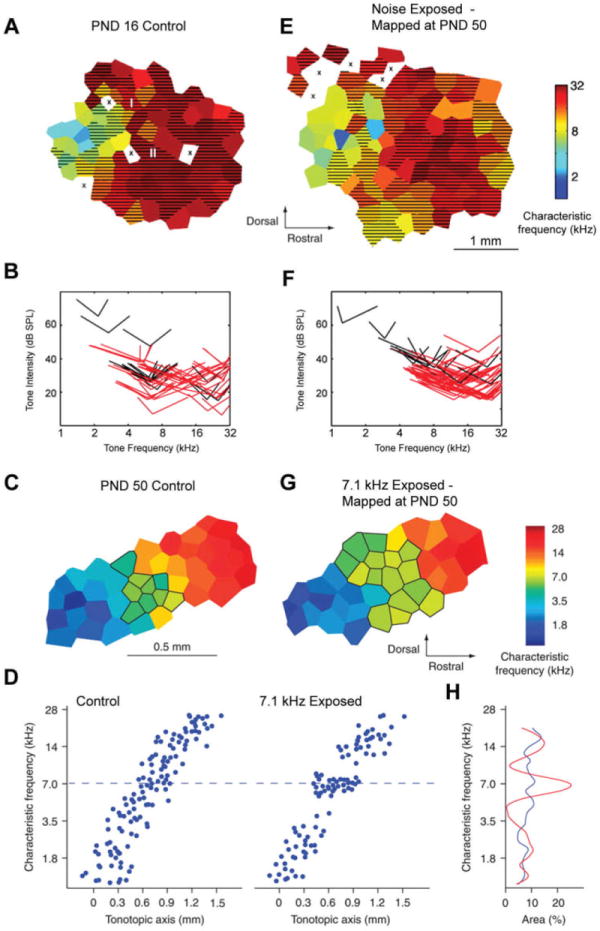
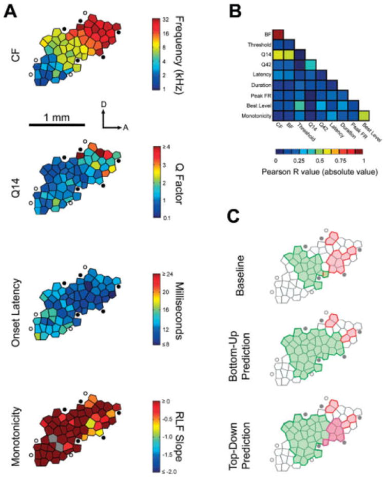
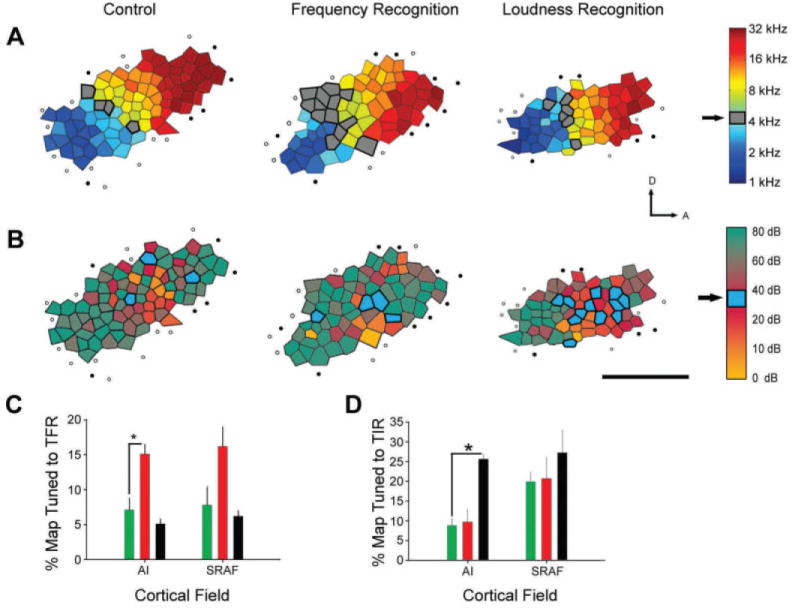
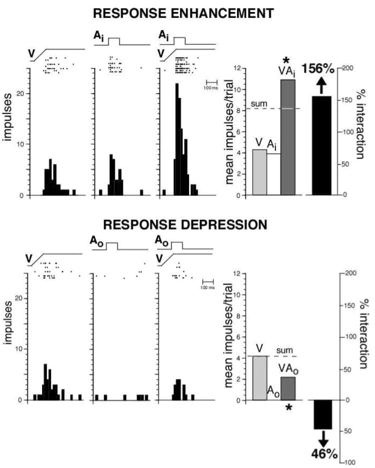
The functional architecture of sensory brain regions reflects an ingenious biological solution to the competing demands of a continually changing sensory environment. While they are malleable, they have the constancy necessary to support a stable sensory percept. How does the functional organization of sensory brain regions contend with these antithetical demands? Here we describe the functional organization of auditory and multisensory (i.e., auditory-visual) information processing in three sensory brain structures: (1) a low-level unisensory cortical region, the primary auditory cortex (A1); (2) a higher-order multisensory cortical region, the anterior ectosylvian sulcus (AES); and (3) a multisensory subcortical structure, the superior colliculus (SC). We then present a body of work that characterizes the ontogenic expression of experience-dependent influences on the operations performed by the functional circuits contained within these regions. We will present data to support the hypothesis that the competing demands for plasticity and stability are addressed through a developmental transition in operational properties of functional circuits from an initially labile mode in the early stages of postnatal development to a more stable mode in the mature brain that retains the capacity for plasticity under specific experiential conditions. Finally, we discuss parallels between the central tenets of functional organization and plasticity of sensory brain structures drawn from animal studies and a growing literature on human brain plasticity and the potential applicability of these principles to the audiology clinic.

Figure 1

Tonotopic map development in normal and abnormal auditory environments. Representative characteristic frequency (CF) maps from auditory cortex of a PND 16 rat (A), a naïve adult (C), a PND 50 young adult reared in continuous white noise (E), and a young adult rat reared in the presence of pulsed 7.1 kHz tones (G). Neurons sampled from the hatched areas had frequency tuning bandwidths measured 20 dB above threshold (BW20s) greater than 1.5 octaves (A and E) Neurons in outlined areas had characteristic frequencies in a range of 7.1 kHz ± 0.2 octaves (C and G). X = unresponsive sites. Note difference in scale bars between top and bottom pairs of maps. B and F: Receptive fields recorded from maps shown in A and E. Distribution of BW10 tuning curve tips from each map, illustrating the CF threshold, and BW10s recorded at each penetration. Red tips denote BW10s greater than 1.5 octaves, D: Characteristic frequency distribution along the tonotopic axis in control and 7.1 kHz-exposed groups. Note the clustering of characteristic frequencies near 7.1 kHz in the 7.1 kHz-exposed animals. H: Percent primary auditory cortex area representing frequencies in a 0.4 octave frequency band. The representations of 7.1 kHz ± 0.2 octaves were significantly larger in tone-exposed animals (red) than they were in control animals (blue). The data shown in panels A, E, B, and F are from Chang and Merzenich (2003). The data shown in panels C, G , D, and H are from Han et al (2007).

Figure 2

Spatial organization of multiple response features within A1. A: Representative A1 map from a naïve adult. The color of each polygon corresponds to the color scale bar for each response feature shown to the right. D and A correspond to dorsal and anterior, respectively. Filled circles indicate unresponsive sites. Open circles represent sound-responsive sites outside A1. Gray polygons indicate sites for which the response parameter of interest could not be calculated. Q14 = the quality factor (CF/bandwidth) measured 14 dB above minimum response threshold. RLF slope = the slope of the rate-level function; more negative values correspond to sites with nonmonotonic intensity-tuned response functions, B: Mutual correlation matrix for ten response features measured in A1 indicating: the absolute value of the Pearson R correlation coefficient for all unique pairs of variables. Note that related response characteristics (e.g., BF and CF or best level and monotonidty) covaried among themselves but not with the other groupings of response characteristics. C: Schematic of the A1 map shown in A illustrating cortical areas preferring midfrequency tones (green polygons) and low intensity tones (red polygons). Relative the pretraining baseline, an adult rat trained o t respond selectively to midfrequency tones would exhibit an expansion of the midfrequency CF representation. The maps below depict the possibility that intensity characteristics of midfrequency tones, though irrelevant to the task, would also be reflected i n the pattern of reorganization (bottom-up prediction), Alternatively, the plasticity could be restricted only to the stimulus dimension that is relevant to the demands of the task (top-down prediction). The data in panels A and B are from Polley et al, 2007.

Figure 3

Task-specific functional reorganization in adult rat A1. Maps for CF (A) and best level (B) are presented for a representative naïve control (left column), a representative rat trained in a frequency recognition task (middle column), and a representative rat trained in a loudness recognition task (right column). A: Gray shaded polygons indicate recording sites with CF values within the trained frequency range (5 kHz ± 0.375 octaves). Filled circles indicate unresponsive sites. Open circles represent sites with sound-driven responses that did not meet the criteria for inclusion in A1. Scale bar = 1 mm. The arrows indicate dorsal (D) and anterior (A) orientations, respectively. B: The same conventions as in A, except that the color within each polygon indicates the best level for neurons at that recording site, rather than CF. Empty polygons indicate recording sites where a best level could not be determined. Blue shaded polygons indicate recording sites with best-level values in the trained intensity rage (35 ± 5 dB SPL). C: Percent of map area within A1 and a secondary auditory field, SRAF, allocated to the trained frequency range (TFR) in naïve control rats (green), rats trained in the frequency recognition task (red), and rats trained in the loudness recognition task (black), D: Percent of map area within A1 and SRAF allocated to the trained intensity range (TIR). Color conventions are the same as C. Asterisks indicate statistically significant differences between groups (p < 0.05). The data are from Polley et al (2006).

Figure 4

Multisensory integration can be divided into two broad operational categories. Response enhancement (top) represents a gain (i.e., increase) in response upon presentation of stimuli in multiple modalities. Rasters and peristimulus time histograms on the left depict the responses of a single multisensory neuron to a visual stimulus alone (V), to an auditory stimulus alone (Ai), and to the combined presentation of these stimuli. Ramps and square waves show the relative timing of the stimuli. Summary bar graphs on the right plot this neuron’s mean response to each of these conditions, as well as the relative gain in response (i.e., 156%) to the multisensory combination. Note that the percent interaction is calculated in this example as [(VAi − V)/V] × 100. In addition, note that, the multisensory response exceeds that predicted by a simple addition of the component unisensory responses. Response depression (bottom) represents a decline in response relative to the best unisensory condition. Here we see that the presentation of an auditory stimulus outside of its receptive field (Ao—contrast this with the Ai condition shown above) results in a significant decline in the visual response.

Figure 5

Multisensory neurons in the cat SC and AES mature over the first four to five months of postnatal life. Graph plots the incidence of multisensory neurons as a percentage of the total neuronal populations in the SC and AES as a function of postnatal age. Note for both structures the absence of multisensory neurons immediately after birth and the gradual rise in their incidence with time. Note also the delay in cortical multisensory maturation as opposed to subcortical maturation. Data adapted from Wallace and Stein, 1997, and Wallace et al, 2006.

Figure 6

Multisensory integration is absent in the earliest multisensory neurons and appears during postnatal development. Shown is representative data from two multisensory SC neurons at two different developmental ages: 20 days postnatal (A, left) and 30 days postnatal (B, right), At the top of each are shown the receptive fields (shading) and locations of the stimuli used in sensory testing (icons). Middle panels show Tasters, histograms, and summary bar graphs depicting the responses to both of the unisensory stimuli and to the multisensory combination. The lines at the top show the relative timing of the stimuli, and the bar graph on the far right in each shows the magnitude of the multisensory interaction (i.e., % integration). At the bottom are shown representative oscillographic traces for a single trial to each of the unisensory stimuli and to the multisensory combination. Note that whereas the neuron in the 20-day-old animal responds to the multisensory combination in a manner virtually identical to its response to the unisensory stimuli, the neuron from the older animal shows a large response enhancement to the stimulus combination, and that this gain exceeds that predicted from the simple summation of the unisensory responses. Data adapted from Wallace and Stein, 1997.

Figure 7

The development of multisensory integration is highly plastic and can be shaped by manipulating early postnatal sensory experience. A: Multisensory interactions as a function of the spatial location of paired visual and auditory stimuli are plotted for two representative SC neurons—one in an animal raised under normal sensory conditions and the other from an animal raised in an environment in which the visual and auditory stimuli were always displaced by 30°. In this representation, the neuron’ responses to the multisensory (i.e., auditory-visual) condition were compared to its responses to the most effective unisensoiy stimulus in order to determine the multi sensory interaction using the formula (M − Umax/Umax) × 100 where M is the multisensory response and Umax is the largest unisensory response (see Stein and Meredith, 1993, for additional detail). For the neuron from the normally reared animal (blue), note that the largest multisensory interactions are seen for pairings in which the stimuli are in close spatial proximity (i.e., 0° and 10°). In contrast, for the animal raised in the spatially disparate environment, the largest interactions are seen for disparities close to those that reflect the early sensory experiences (i.e., 30°, red). Blue and red shading show the spatial “window” for multisensory interactions in these two neurons, in which the stimulus combination results in a significant change in activity. B: Multisensory interactions as a function of the temporal interval between paired visual and auditory stimuli are plotted for three representative SC neurons—one in an animal raised under normal sensory conditions (blue), one from an animal raised in an environment in which the visual and auditory stimuli were always temporally offset by 100 msec (red), and one from an animal raised in an environment in which the visual and auditory stimuli were always temporally offset by 250 msec (green). Note that in the normally reared animal the largest multisensory interactions are seen when the visual stimulus precedes the auditory stimulus by 100 msec. In the neuron from the 100 msec temporal disparity reared animal this interval is increased to 200 msec. In comparison, in the 250 msec temporal disparity reared animal no multisensory interactions are seen.

Figure 8

A simple model of the enlargement in the temporal window of multisensory integration in dyslexic readers. Shown at the top in yellow shading is the temporal window of multisensory binding in a typical reader, Note in panel A that if a visual (V) and auditory (A) event occur within this window, they are bound as a single perceptual entity. In contrast, with additional temporal separation (B), they are processed as separate events. At the bottom is shown the extended temporal window proposed for dyslexic readers, and the consequent impact of this window on the binding of visual and auditory events. Adapted from Hairston et al, 2005.

References

1. Ahissar M, Hochstein S. Attentional control of early perceptual learning. Proc Natl Acad Sci U S A. 1993;90(12):5718–5722. - PMC - PubMed
1. Bakin JS, South DA, Weinberger NM. Induction of receptive field plasticity in the auditory cortex of the guinea pig during instrumental avoidance conditioning. Behav Neurosci. 1996;110(5):905–913. - PubMed
1. Bakin JS, Weinberger NM. Classical conditioning induces CS-specific receptive field plasticity in the auditory cortex of the guinea pig. Brain Res. 1990;536(1-2):271–286. - PubMed
1. Bakin JS, Weinberger NM. Induction of a physiological memory in the cerebral cortex by stimulation of the nucleus basalis. Proc Natl Acad Sci U S A. 1996;93(20):11219–11224. - PMC - PubMed
1. Bao S, Chan VT, Merzenich MM. Cortical remodelling induced by activity of ventral tegmental dopamine neurons. Nature. 2001;412(6842):79–83. - PubMed