Adaptable mechanisms that regulate the contrast response of neurons in the primate lateral geniculate nucleus

Abstract

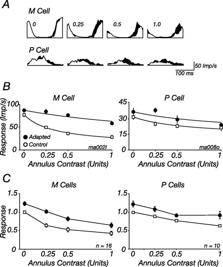
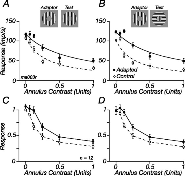
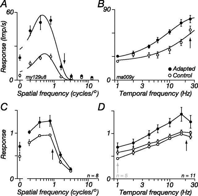
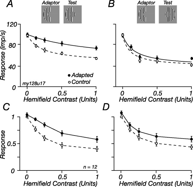
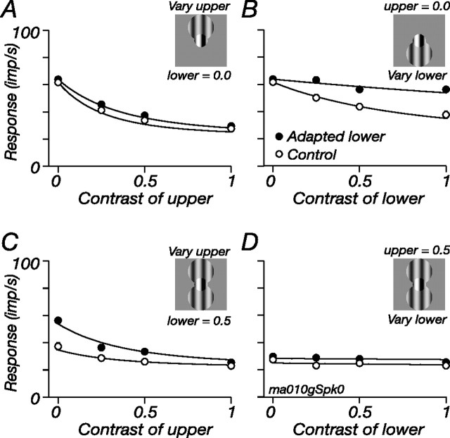
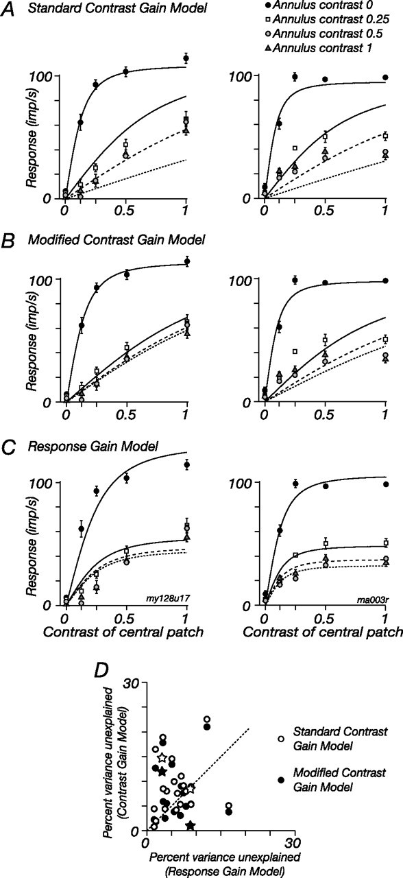
The response of the classical receptive field of visual neurons can be suppressed by stimuli that, when presented alone, cause no change in the discharge rate. This suppression reveals the presence of an extraclassical receptive field (ECRF). In recordings from the lateral geniculate nucleus (LGN) of a New World primate, the marmoset, we characterize the mechanisms that contribute to the ECRF by measuring their spatiotemporal tuning during prolonged exposure to a high-contrast grating (contrast adaptation). The ECRF was strongest in magnocellular cells, where contrast adaptation reduced suppression from the ECRF: adaptation of the ECRF transferred across spatial frequency, temporal frequency, and orientation, but not across space. This implies that the ECRF of LGN cells comprises multiple adaptable mechanisms, each broadly tuned but spatially localized, and consistent with a retinal origin. Signals from the ECRF saturated at high contrasts, and so adaptation of one part of the ECRF brought into its operating range signals from other parts of the visual field. Although the ECRF is adaptable, its major impact during contrast adaptation to a spatially extended pattern was to reduce visual response and hence reduce a neuron's susceptibility to contrast adaptation; in normal viewing, a major role of the ECRF might be to protect visual sensitivity in scenes dominated by high contrast.

Figure 1.

Spatial summation in P and M cells in marmoset LGN. A, M cell. B, P cell. Each curve plots the amplitude of response at the frequency of stimulation (F1). The filled symbols show responses to drifting gratings presented within a circular patch, the outer diameter of which was varied. The open symbols show responses to an annular patch of the same drifting grating, the inner diameter of which was varied. The shaded symbols show responses to an annulus that contained a uniform field modulated in time: the inner diameter of the annulus was varied. For both the P and M cell, the inner diameter of the annular grating had to be <0.5° to elicit a response, whereas the uniform annuli evoked responses at most inner diameters. For the P cell, responses to circular patches of drifting gratings rapidly increase with patch size and then asymptote. For the M cell, responses to the patches first increase with patch size, then decrease; this decrease (suppression) reveals the presence of an ECRF. Temporal frequency, 5 Hz; contrast, 0.5; spatial frequency, 2 cycles/° (A) or 3 cycles/° (B). In this and all subsequent figures, the error bars show ±1 SEM.

Figure 2.

Contrast adaptation reduces the contrast sensitivity of M cells in marmoset LGN. A, Peristimulus time histograms (PSTHs) showing modulation of the discharge in response to a grating drifting at 5.5 Hz, sampled in 1 s epochs during adaptation to a high-contrast grating of optimal size and spatial frequency (shaded histograms, Adapted) or a blank screen (open histograms, Control). PSTHs are shown for four contrasts of the grating for one M cell (top) and one P cell (bottom). B, Response amplitude (F1) as a function of stimulus contrast, for tests presented during adaptation to a high-contrast grating (filled symbols) or blank screen (open symbols). The same cells as in A are shown. Solid lines show best-fitting predictions of Equations 1–3, where for each cell only σ_c was allowed to vary. Temporal frequency, 5.5 Hz; diameter, 0.5° (P cell) or 0.4° (M cell); spatial frequency, 3 cycles/° (P cell) or 3.2 cycles/° (M cell). C, Average for all M and P cells in our sample. (1 M cell was tested at different contrasts and is excluded from the plot). Responses of each cell were normalized to the maximum obtained in the control state before averaging.

Figure 3.

Contrast adaptation reduces the difference in contrast gain of P and M cells. Contrast gain (obtained from Eq. 1: G/σ_c) of 14 P cells (filled symbols) and 18 M cells (open symbols) for gratings of optimal size and spatial frequency, in control conditions (abscissa) and during adaptation to a high-contrast grating of the same configuration (ordinate), is shown. Arrows on the ordinate and abscissa show the geometric mean contrast gain for P cells (filled arrows) and M cells (open arrows). In the control state, this average gain of M cells was 382 imps/s/[unit contrast], and in the adapted state it was 72. For P cells, these values were 72 and 45, respectively.

Figure 4.

The impact of contrast adaptation depends on the size and contrast of the adapting grating. A, Contrast response for a patch of drifting grating of optimal diameter (0.3°) during adaptation to a patch of high-contrast grating of diameter 8° (filled symbols) or to a blank screen (open symbols). B, Same as A, but the adapting grating was smaller (diameter 0.3°) and of high contrast (contrast, 1.0; filled symbols) or low contrast (contrast, 0.2; shaded symbols). Solid lines show best-fitting predictions of Equations 1–3, where for each adaptor only σ_c was allowed to vary. Temporal frequency, 5.5 Hz; spatial frequency, 1.8 cycles/°. The low-contrast adaptor evoked 39.6 imp/s; the large high-contrast adaptor evoked 46.0 imp/s; the small high-contrast adaptor evoked 64.0 imp/s.

Figure 5.

Contrast adaptation reduces suppression from the ECRF. A, Peristimulus time histograms (PSTHs) showing modulation of the discharge in response to a central patch of grating drifting at 5.5 Hz, in the presence of a surrounding annuli drifting at 8.3 Hz. Responses during adaptation to a high-contrast annulus grating (shaded histograms, Adapted) or a blank screen (open histograms, Control) are shown. PSTHs are shown for four contrasts of the annulus grating for one M cell (top) and one P cell (bottom). B, Response amplitude at the temporal frequency of the central patch (F1) as a function of annulus contrast, for tests presented during adaptation to a high-contrast annulus (filled symbols) or blank screen (open symbols). The same cells as in A, which are also shown in Figure 2, are shown. Solid lines show best-fitting predictions of Equations 1–3, where for each cell only σ_s was allowed to vary. Contrast of central patch, 0.5; diameter of central patch, 0.5° (P cell) or 0.4° (M cell); spatial frequency of central and annular patch, 3 cycles/° (P cell) or 3.2 cycles/° (M cell). C, Average for all M and P cells in our sample. (1 M cell was tested at different contrasts and is excluded from the plot). Responses of each cell were normalized to the maximum obtained in the control state before averaging.

Figure 6.

Adaptation of the ECRF transfers across orientation. A, B, Response of an M cell to a central patch in the presence of annuli of the same orientation as that patch (A), or the orthogonal orientation (B), in the control state and during adaptation to an annulus of the same orientation as the patch. Central patch contrast, 0.5; diameter, 0.6°; spatial frequency, 0.8 cycles/°. C, D, Average response of 12 cells in the control state and during annular adaptation; the response of each cell was normalized to the maximum obtained in the control state before averaging. C, Test annuli at the same orientation as the patch and the adaptor. D, Test annuli orthogonal to the adaptor. Conventions are as in Figure 5B.

Figure 7.

Adaptation of the ECRF transfers across spatial and temporal frequency. A, Response of an M cell as a function of spatial frequency for a large (diameter, 8°) patch of drifting grating, in the control state and during adaptation to an annular grating of high spatial frequency. Contrast, 0.2; temporal frequency, 5 Hz. B, Response of another M cell as a function of temporal frequency for a large patch of grating, in the control state and during adaptation to an annular grating of high temporal frequency. Contrast, 0.25; spatial frequency, 1 cycle/°. C, Average spatial frequency tuning curves of a subset of M cells where the annular adaptor was a grating of spatial frequency between 0.8 and 1 cycle/° (μ = 0.95; SD, 0.14). D, Average response of all M cells during adaptation to an annular grating of optimal spatial frequency, drifting at 16 or 25 Hz (n = 11; filled symbols). A subset (n = 5) was also tested during annular adaptation to a grating that drifted at 1 Hz (shaded symbols). The average control response (open symbols) of this subset could not be distinguished from the average response of all 11 cells and is omitted for clarity. Arrows show the adapting frequencies, which were 2 cycles/° and 8.3 Hz (A) or 1 cycle/° and 25 Hz (B). Smooth lines show the best predictions of the descriptive model described in Results. In C and D, the response of each cell was normalized to the maximum obtained in the control state before averaging.

Figure 8.

Adaptable ECRF mechanisms are spatially localized. The response of an M cell to a central patch in the presence of varying contrasts of half an annulus (hemifield), in the control state (open symbols) and during adaptation to a high-contrast hemifield (filled symbols). A, Responses in the control and adapted state for the hemifield that was adapted. B, Same as in A, but for the unadapted hemifield. Central patch contrast, 0.5; diameter, 1°; spatial frequency, 1 cycle/°. C, D, Average response of 12 cells in the control state and during adaptation to an annular hemifield; the response of each cell was normalized before averaging. C, Test stimuli in the same hemifield as the adaptor. D, Test stimuli in the other hemifield. Conventions are as in Figure 5B.

Figure 9.

Pooled signals of adaptable ECRF subunits are subject to a compressive nonlinearity. For a full description of the figure, see Results. A central test grating (contrast, 0.25) abutted two discs whose contrast varied independently, the spatial arrangement of which is indicated by the insets. Each panel shows the modulated response at the frequency of stimulation of the central patch (5.5 Hz). A, C, Response as a function of the contrast of the grating in the upper disc. A, The lower disc was held at zero contrast. C, The lower disc was a drifting grating (8.3 Hz) of contrast 0.5. B, D, Response as a function of the contrast of the grating in the lower disc. B, The upper disc was held at zero contrast. D, The upper disc was a drifting grating of contrast 0.5. In all panels, the open symbols show responses in the control state, and filled symbols show responses during adaptation to a high-contrast grating confined to the lower disc. Lines show the predictions of the model described in Results (Eq. 4). Central patch diameter, 0.7°; disc diameters, 1.4°; spatial frequency of all gratings, 0.8 cycles/°.

Figure 10.

Adaptation of the ECRF changes spatial summation. Two examples showing how the tuning for the diameter of a patch of drifting grating is changed by adaptation to an annular grating are shown. A, M cell showing generalized increase of response at large patch diameters. B, M cell appearing to show a change in the area over which suppressive signals are gathered. Smooth lines show the best-fitting predictions of the model described in Results. Conventions are as in Figure 5B. Contrast, 0.5; temporal frequency, 5.5 Hz; spatial frequency, 3.2 cycles/° (A) or 2 cycles/° (B).

Figure 11.

Comparison of contrast–gain and response–gain models of the ECRF. A, The left panels show the modulated response of one M cell, and the right panels show the response of a second M cell, at the drift frequency (5.5 Hz) of a central patch of sinusoidal grating. The central patch abutted an annular grating that drifted at 8.3 Hz. The four sets of data points in each panel show response as a function of the patch contrast, for each of four annulus contrasts. The lines show the predictions of the standard contrast gain model of the ECRF (Eq. 5 in Results). B, Same data as in A. The lines show the predictions of a modified contrast gain model, where the ECRF signal was subject to a compressive nonlinearity. C, Same data as in A and B. The lines show the predictions of the response gain model. D, The open symbols compare the response variance left unexplained by the response gain model (C) and the standard contrast gain model (A) for all cells (n = 22). The filled symbols compare the response gain model and the modified contrast gain model (B) for the same cells. The stars plot the cells shown in A–C.

References

1. Alitto HJ, Usrey WM. Origin and dynamics of extraclassical suppression in the lateral geniculate nucleus of the macaque monkey. Neuron. 2008;57:135–146. - PMC - PubMed
1. Angelucci A, Levitt JB, Walton EJ, Hupe JM, Bullier J, Lund JS. Circuits for local and global signal integration in primary visual cortex. J Neurosci. 2002;22:8633–8646. - PMC - PubMed
1. Baccus SA, Meister M. Fast and slow contrast adaptation in retinal circuitry. Neuron. 2002;36:909–919. - PubMed
1. Barlow HB. Summation and inhibition in the frog's retina. J Physiol. 1953;119:69–88. - PMC - PubMed
1. Barlow HB, Hill RM. Evidence for a physiological explanation of the waterfall phenomenon and figural after-effects. Nature. 1963;200:1345–1347. - PubMed
Publication types
LinkOut - more resources