Clinical applications of magnetoencephalography

Abstract

Magnetoencephalography (MEG), in which magnetic fields generated by brain activity are recorded outside of the head, is now in routine clinical practice throughout the world. MEG has become a recognized and vital part of the presurgical evaluation of patients with epilepsy and patients with brain tumors. We review investigations that show an improvement in the postsurgical outcomes of patients with epilepsy by localizing epileptic discharges. We also describe the most common clinical MEG applications that affect the management of patients, and discuss some applications that are close to having a clinical impact on patients.

Figure 1

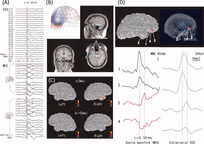
Localization of epileptic spikes. (A) Simultaneously acquired EEG (top) and MEG (bottom) signals from a patient with epilepsy. An epileptic spike is seen in MEG sensors over the right temporal and frontal regions. (B) An equivalent current dipole (ECD) computed at the peak of the spike (“0 ms”; the corresponding isocontour map of the MEG data, with the ECD as a green arrow, is shown at top left) is localized in the temporal lobe (blue dots superimposed on the anatomical MRI). (C) Distributed source estimates, the noise‐normalized minimum‐norm estimate (MNE), also known as dynamic statistical parametric map (dSPM), for the MEG data are displayed on the cortical surface representation reconstructed from anatomical MRI. The source estimates suggest that the activity propagates from a right temporal region (“0 ms”) to the right frontal region (“50 ms”). (D) Comparison of MEG data with ECoG. The left panel shows the estimated MEG source waveforms (MNE) at four locations (“1” and “2” temporal, “3” and “4” frontal). The right panel shows the ECoG of an epileptic spike at corresponding locations. The MEG and ECoG are consistent in suggesting temporal activity propagating to the frontal lobe over a 50‐ms time period.

Figure 2

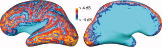
Relative signal‐to‐noise ratio (SNR) of cortical sources in MEG and EEG. The color coding indicates regions where the expected SNR of a focal cortical sources is larger in MEG than in EEG (red and yellow) or vice versa (blue). Lateral (left) and medial (right) view of an inflated representation of the left‐hemisphere cerebral cortex is shown. Maps like this help to understand why epileptic spikes and other cortical activity may at times be detectable only in MEG or only in EEG but not necessarily in both. SNR was calculated from a forward model as the logarithm of the sum across all sensors of the ratio of measured signal from a unit source divided by the noise variance on the sensor, divided by the number of sensors (from Goldenholz et al., Hum Brain Mapp, 2009, 30, 1077–1086, © Wiley‐Liss, reproduced by permission).

Figure 3

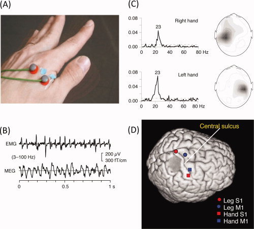
Motor cortex localization using MEG‐EMG coherence. (A) Placement of the surface bipolar electromyogram (EMG) electrodes on the first interossesous muscle. (B) Waveforms of EMG and MEG (from a sensor over the motor cortex). (C) Coherence between the EMG and MEG signals as a function of frequency. (D) Locations of equivalent current dipoles in the right primary motor cortex, obtained by localizing the peak coherence (∼20 Hz). (B) and (C) From Salenius et al., J Neurophysiol, 1997, 77, 3401–3405, © American Physiological Society, reproduced by permission. (D) From Makela et al., Hum Brain Mapp, 2001, 12, 180–192, © Wiley‐Liss, reproduced by permission.

Figure 4

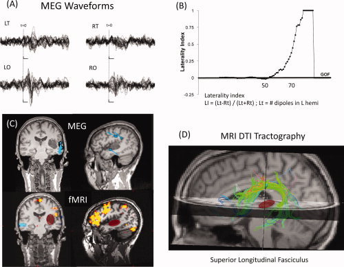
Multimodal imaging of language (MEG, fMRI, and DTI). (A) MEG waveforms for left and right temporal (LT and RT, respectively) and occipital (LO, RO) sensors, showing evoked responses to a language task. (B) Laterality index as a function of goodness of fit (GOF) of a sequential equivalent current dipole (ECD) fit to the MEG data, suggesting left‐hemisphere dominance. (C) Locations of the ECDs for the MEG data (top) and functional MRI (bottom) for a visual reading task, displayed in coronal and sagittal slices of an anatomical MRI. Note the cluster of MEG dipoles in the posterior superior temporal gyrus, presumably including Wernicke's area. Functional MRI shows largest activation in the inferior lateral left frontal cortex. The location of a tumor in the left temporal lobe is highlighted with the red oval. (D) MRI tractography showing the superior longitudinal fasciculus (SLF), which includes the arcuate fasciculus, that connects temporal and frontal language areas. Note that the tumor (red) does not interrupt or displace the SLF white matter fiber bundle. (Case courtesy of Drs. Emad Eskandar, M.D., Ph.D. and Andrew Cole, M.D., of Massachusetts General Hospital).

Figure 5

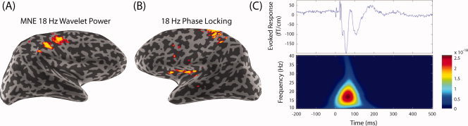
Spectral spatiotemporal mapping of the somatosensory system. (A) The 18‐Hz wavelet‐based spectral spatiotemporal maps using minimum‐norm estimate (MNE) in the right hemisphere (left‐hand median nerve stimulation). (B) Transhemispheric phase locking between the primary somatosensory cortex (SI) and the contralateral secondary somatosensory cortex (SII). Based on the maximal power dipole in the right hemisphere, a left‐hemisphere phase‐locking (phase synchrony) map shows 18‐Hz synchrony of the right SI and left SII. (C) For the somatosensory‐evoked response by median nerve stimulation, the evoked response is found in the contralateral hemisphere with an initial peak at ∼20 ms (upper panel). The spectrogram shows a burst centered around 18 Hz and peaking in magnitude at about 85 ms after the mean nerve was stimulated (lower panel) (From Lin et al., Neuroimage, 2004, 23, 582–595, © Academic Press, reproduced by permission).