Syndromic surveillance: STL for modeling, visualizing, and monitoring disease counts

Abstract

Background: Public health surveillance is the monitoring of data to detect and quantify unusual health events. Monitoring pre-diagnostic data, such as emergency department (ED) patient chief complaints, enables rapid detection of disease outbreaks. There are many sources of variation in such data; statistical methods need to accurately model them as a basis for timely and accurate disease outbreak methods.

Methods: Our new methods for modeling daily chief complaint counts are based on a seasonal-trend decomposition procedure based on loess (STL) and were developed using data from the 76 EDs of the Indiana surveillance program from 2004 to 2008. Square root counts are decomposed into inter-annual, yearly-seasonal, day-of-the-week, and random-error components. Using this decomposition method, we develop a new synoptic-scale (days to weeks) outbreak detection method and carry out a simulation study to compare detection performance to four well-known methods for nine outbreak scenarios.

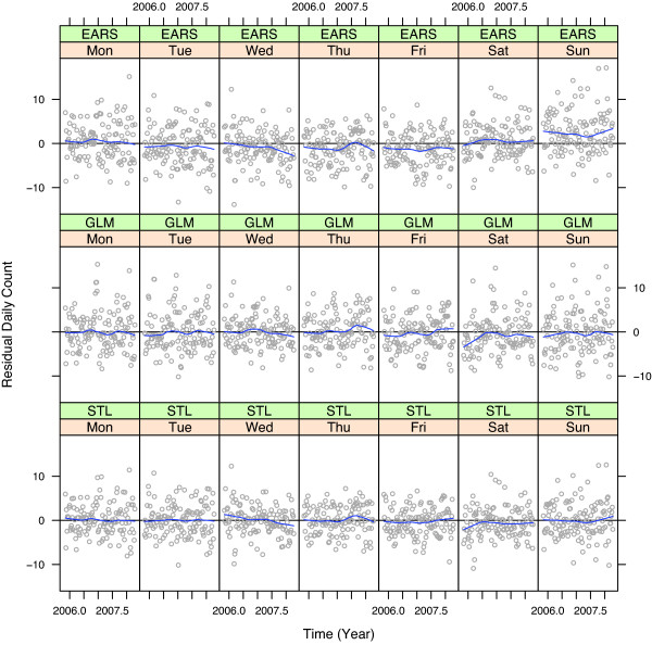
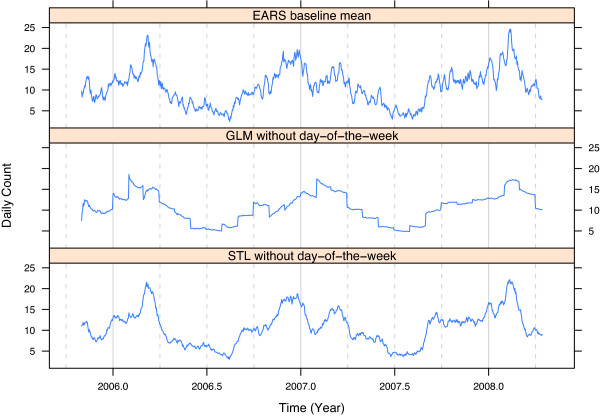
Result: The components of the STL decomposition reveal insights into the variability of the Indiana ED data. Day-of-the-week components tend to peak Sunday or Monday, fall steadily to a minimum Thursday or Friday, and then rise to the peak. Yearly-seasonal components show seasonal influenza, some with bimodal peaks.Some inter-annual components increase slightly due to increasing patient populations. A new outbreak detection method based on the decomposition modeling performs well with 90 days or more of data. Control limits were set empirically so that all methods had a specificity of 97%. STL had the largest sensitivity in all nine outbreak scenarios. The STL method also exhibited a well-behaved false positive rate when run on the data with no outbreaks injected.

Conclusion: The STL decomposition method for chief complaint counts leads to a rapid and accurate detection method for disease outbreaks, and requires only 90 days of historical data to be put into operation. The visualization tools that accompany the decomposition and outbreak methods provide much insight into patterns in the data, which is useful for surveillance operations.

Figure 1

STL decomposition for respiratory square root daily counts. Respiratory square root daily counts and four components of variation of the STL decomposition for an Indiana emergency department (ED). The four components sum to the square root counts. The solid vertical lines show January 1 and the dashed vertical lines show April 1, July 1, and October 1.

Figure 2

Outbreak sample. Randomly generated outbreak of 76 cases injected according to the Sartwell model [26] is shown by the histogram. The lognormal density of the model multiplied by 76 is shown by the curve. The parameters of the lognormal are the mean, ζ = 2.401, and the standard deviation, σ = 0.4626, both on the natural log scale.

Figure 3

Day-of-the-week component. Day-of-the-week component, D_t, for square root respiratory counts for 30 Indiana EDs. The general pattern is U-shaped with a Monday or Sunday maximum and a Thursday or Friday minimum.

Figure 4

Yearly-seasonal component. Yearly-seasonal component, S_t, for square root respiratory daily counts for 30 Indiana EDs. Overall, patterns are similar, but detailed behavior varies with unimodal and bimodal peaks, different times of onset of yearly-seasonal disease, and different times of disease peaks.

Figure 5

Inter-annual component. Inter-annual component, T_t, for respiratory square root counts for 30 Indiana EDs. Each component has been centered around zero to protect anonymity. The long-term trend for each ED is either nearly constant or has a small increase due to a growing patient population.

Figure 6

Normal probability plots for N_t. Normal quantile plots for the noise component, N_t, of the square root respiratory counts for 30 EDs. The sample distribution of the noise is well approximated by the normal distribution. This is a result of the square root transformation of the counts.

Figure 7

Outbreak simulation results. Outbreak detection simulation results. The false positive rate was set empirically for each method and baseline to be 0.03. For each baseline, the STL method detects more than 10% more outbreaks than the other methods at the smallest magnitude.

Figure 8

Observed false positive rates for STL and GLM. Quantile plots of observed false positive rates for the STL and GLM methods based on a theoretical false positive rate of 0.03, from respiratory counts for each of the 30 EDs. The dashed lines represent the median value for each method.

Figure 9

Residuals for model fits. Residuals for model fits to daily respiratory counts for one ED. The EARS residuals are the observed count minus the 7 day baseline mean with lag 2. The GLM and STL residuals are obtained from the model predicted values. The smooth curve is the local mean of the residuals.

Figure 10

Residuals by day-of-the-week. Residuals for model fits to daily respiratory counts for one ED, by day-of-the-week. The smooth curve is the local mean of the residuals.

Figure 11

Fitted components. Fitted components for daily respiratory counts for one ED. The EARS fitted value at day t is the the 7 day baseline mean with lag 2. The GLM and STL fitted values are the predicted values from fitting the models up to day t but with the day-of-the-week components removed to make comparison with the variability of the EARS fitted values commensurate.

References

1. Burkom H. Development, adaptation, and assessment of alerting algorithms for biosurveillance. Johns Hopkins APL Technical Digest. 2003;24(4):335–342.
1. Burkom H, Murphy S, Shmueli G. Automated time series forecasting for biosurveillance. Stat in Med. 2007;26(22):4202–4218. doi: 10.1002/sim.2835. - DOI - PubMed
1. Reis B, Mandl K. Time series modeling for syndromic surveillance. BMC Med Inform Decis Mak. 2003;3:2. doi: 10.1186/1472-6947-3-2. - DOI - PMC - PubMed
1. Hutwagner L, Thompson W, Seeman G, Treadwell T. The bioterrorism preparedness and response Early Aberration Reporting System (EARS) J Urban Health. 2003;80:i89–i96. - PMC - PubMed
1. Wallenstein S, Naus J. Scan statistics for temporal surveillance for biologic terrorism. MMWR Morb Mortal Wkly Rep. 2004;53 Suppl:74–78. - PubMed
Publication types