Prediction of the rotational tumbling time for proteins with disordered segments

Abstract

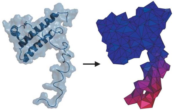
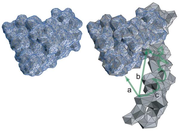
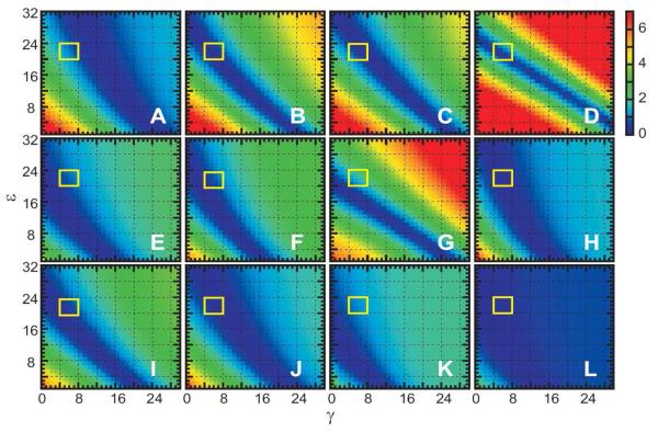
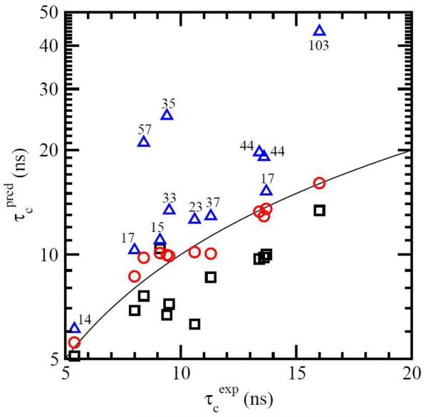
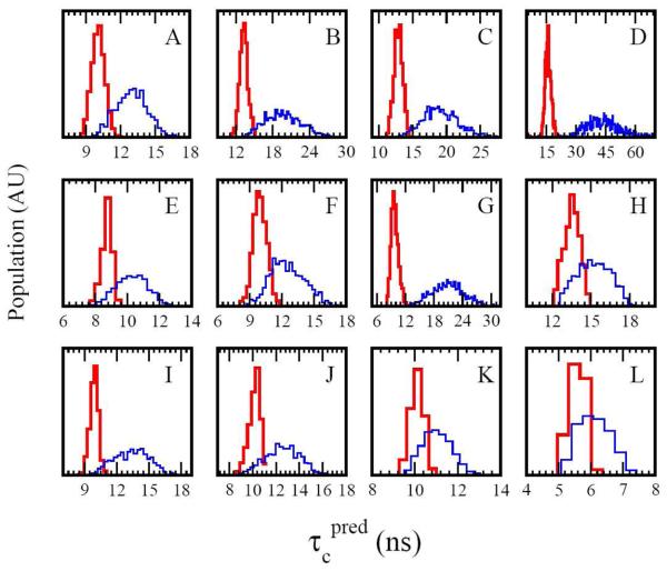
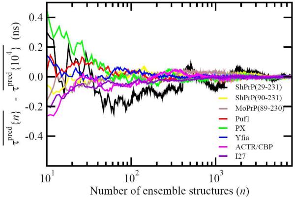
For well-structured, rigid proteins, the prediction of rotational tumbling time (tau(c)) using atomic coordinates is reasonably accurate, but is inaccurate for proteins with long unstructured sequences. Under physiological conditions, many proteins contain long disordered segments that play important regulatory roles in fundamental biological events including signal transduction and molecular recognition. Here we describe an ensemble approach to the boundary element method that accurately predicts tau(c) for such proteins by introducing two layers of molecular surfaces whose correlated velocities decay exponentially with distance. Reliable prediction of tau(c) will help to detect intra- and intermolecular interactions and conformational switches between more ordered and less ordered states of the disordered segments. The method has been extensively validated using 12 reference proteins with 14 to 103 disordered residues at the N- and/or C-terminus and has been successfully employed to explain a set of published results on a system that incorporates a conformational switch.

Figure 1

Modeling the surface of an ensemble structure by the boundary elements. In the left, the ribbon diagram and the molecular surface are superimposed for an ensemble structure from the mouse prion protein (residues 89-230) which has 38 and 6 disordered residues at N- and C- terminus, respectively. In the right hand panel, the boundary elements (triangular patches) representing the molecular surface are illustrated. The factor for correlated velocity (eq. 11) is displayed on each surface patch by color gradient (blue:1→red:0). Note that the surface patches on the ordered part are blue and those on the disordered N terminus become increasingly red as their distances from the ordered part increase.

Figure 2

Defining the rigid and instantaneous surfaces and their correlation distance (δ). A rigid surface (left, blue edges) which encloses a least set of common atoms within the heterogeneous ensemble structures and an instantaneous surface (right, black edges) which encloses one member of the ensemble structures superimposed on the rigid surface are illustrated for an ensemble structure of the mouse prion protein (residues 89-230). The molecular surfaces are modeled by a group of triangular patches for the boundary element calculations (2,400 and 1,200 triangular surface elements are displayed here for the rigid and instantaneous surfaces, respectively). The velocity of an instantaneous surface patch is hypothesized to be correlated with that of the closest rigid surface patch by some factor which decays with distance (δ) between two surface patches (eq. 11) (a). Alternatively, a spatial distance (b) or residue number distance (c) to the beginning of the flexible part may be used for the distance, δ. For the distances b and c, each surface element on both the rigid and instantaneous surfaces is correlated with a specific residue based on the atomic coordinates in the relevant member of the disordered ensemble.

Figure 3

Predictions of rotational correlation times (τ_c =D_R⁻¹) with different sets of γ and ε parameters (eq. 11). |τ_c^pred-τ_c^exp| is shown as color gradient (blue:0 ns → red:>7 ns). The consensus γ and ε parameters range is indicated by the yellow box. (A-L) 12 reference proteins, with the number of disordered residues indicated. (A) ACTR(1018-1088)/CBP(2059-2117):37, (B) MoPrP(89-230):44, (C) ShPrP(90-231):44, (D) ShPrP(29-231):103, (E) I27(1-103):17, (F) PUF1(1-106):35, (G) PX(474-568):57, (H) ttRNH(1-166):17, (I) IGFBP-6(1-107):33, (J) Yfia(1-113):23, (K) IIAglc(1-162):15, (L) VMIP-II(1-74):14.

Figure 4

Comparison of predicted and experimental correlation times. Predicted tumbling times (τ_c^pred) from the empirical Stokes-Einstein method (black square), conventional boundary element method with rigid assumption (blue triangle), and the method described in this study (red circle) are compared with the experimental data (τ_c^exp). The solid line represents perfect agreement between τ_c^pred and τ_c^exp. The number of disordered residues for each protein is indicated near the triangle symbol. A semi-log scale is used for the y-axis to cover the wide range of τ_c^pred.

Figure 5

Distribution of the predicted rotational correlation times τ_c^pred for 1,000 ensemble structures. Red histograms display the distribution of τ_c^pred from the ensemble approach to the boundary element method using two layers of molecular surfaces and their correlated velocity relation. For comparison, the distribution of τ_c^pred from the conventional boundary element method assuming each ensemble structure is rigid is displayed in blue histograms. The x-axis shows the rotational correlation time in ns and the bin size is 0.3 ns in all histograms. The y-axis is in arbitrary units and represents the population at each τ_c^pred bin. (A) ACTR(1018-1088)/CBP(2059-2117), (B) MoPrP(89-230), (C) ShPrP(90-231), (D) ShPrP(29-231), (E) I27(1-103), (F) PUF1(1-106), (G) PX(474-568), (H) ttRNH(1-166), (I) IGFBP-6(1-107), (J) Yfia(1-113), (K) IIAglc(1-162), (L) VMIP-II(1-74).

Figure 6

Convergence of the predicted rotational correlation time (τ_c^pred). The prediction was made from the ensemble approach to the boundary element method using two layers of molecular surfaces and their correlated velocity relation. The difference between the τ_c^pred averaged over n ensemble structures $\left(\stackrel{‒}{{{\tau }_{\mathrm{c}}}^{\text{pred}}\left\{n\right\}}\right)$ and the τ_c^pred averaged over 10⁴ ensemble structures $\left(\stackrel{‒}{{{\tau }_{\mathrm{c}}}^{\text{pred}}\left\{{10}^4\right\}}\right)$ is plotted as a function of the number of ensemble structures (n). As the number of ensemble structures increases, the difference approaches toward zero, indicating convergence.

References

1. Halle B, Davidovic M. Proc. Natl. Acad. Sci U. S. A. 2003;100:12135–12140. - PMC - PubMed
1. Kirkwood JG, Riseman J. J. Chem. Phys. 1948;16:565–573.
1. Bloomfield VA. Science. 1968;161:1212–1219. - PubMed
1. Garcia de la Torre J, Huertas ML, Carrasco B. J. Magn Reson. 2000;147:138–146. - PubMed
1. Youngren GK, Acrivos A. J. Fluid Mech. 1975;69:377–403.
Publication types