Granger causality vs. dynamic Bayesian network inference: a comparative study

Abstract

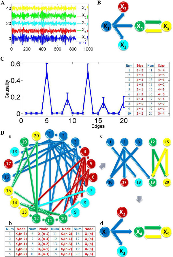
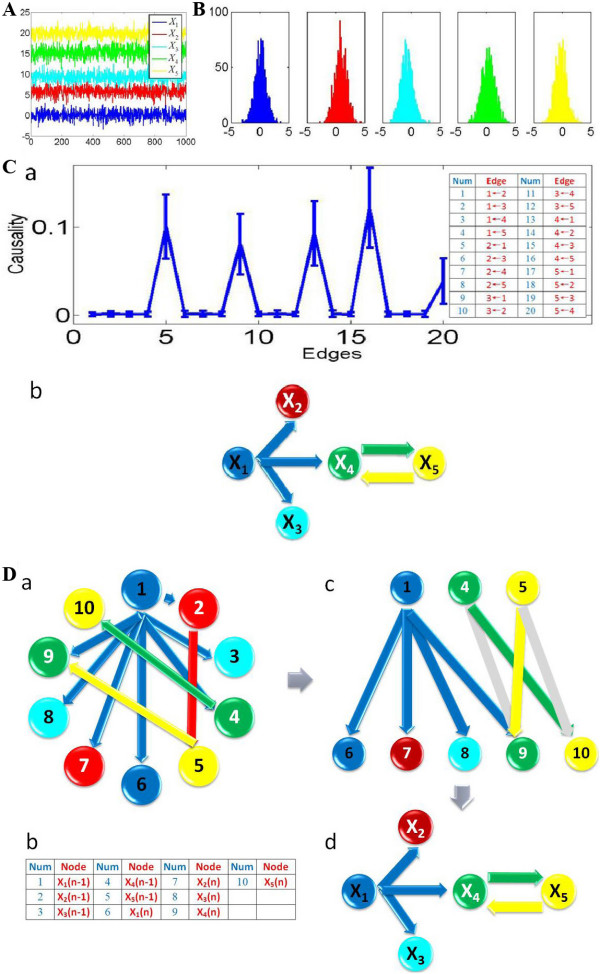
Background: In computational biology, one often faces the problem of deriving the causal relationship among different elements such as genes, proteins, metabolites, neurons and so on, based upon multi-dimensional temporal data. Currently, there are two common approaches used to explore the network structure among elements. One is the Granger causality approach, and the other is the dynamic Bayesian network inference approach. Both have at least a few thousand publications reported in the literature. A key issue is to choose which approach is used to tackle the data, in particular when they give rise to contradictory results.

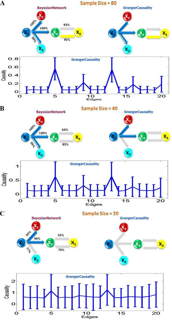
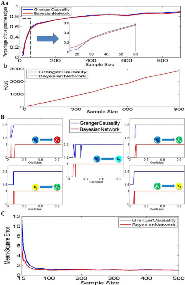
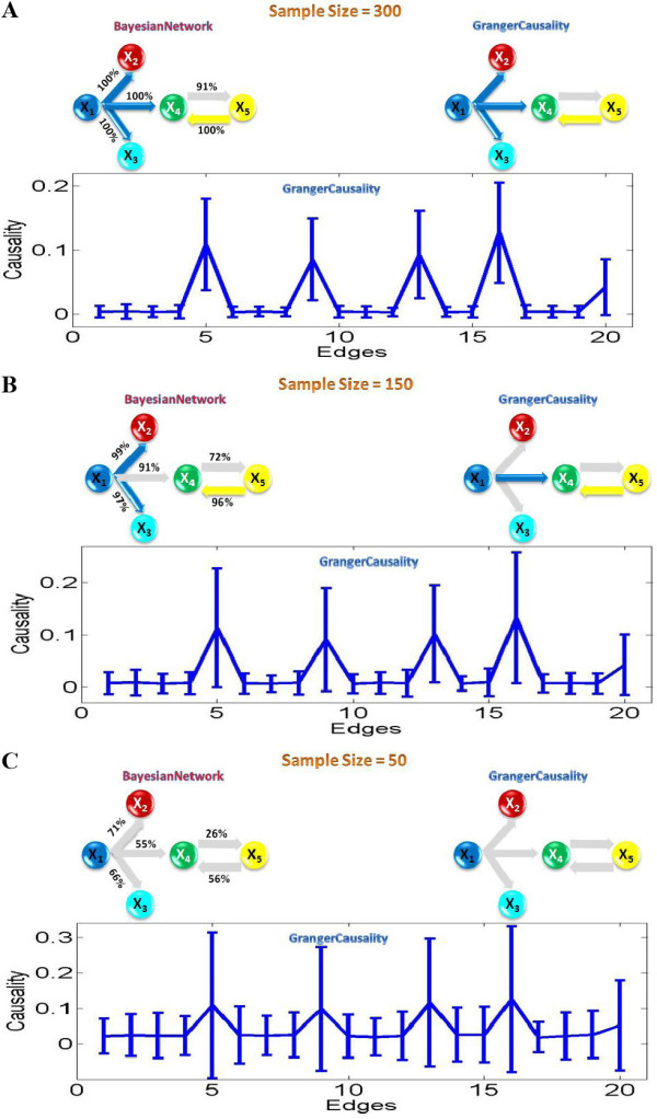
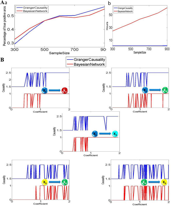
Results: In this paper, we provide an answer by focusing on a systematic and computationally intensive comparison between the two approaches on both synthesized and experimental data. For synthesized data, a critical point of the data length is found: the dynamic Bayesian network outperforms the Granger causality approach when the data length is short, and vice versa. We then test our results in experimental data of short length which is a common scenario in current biological experiments: it is again confirmed that the dynamic Bayesian network works better.

Conclusion: When the data size is short, the dynamic Bayesian network inference performs better than the Granger causality approach; otherwise the Granger causality approach is better.

Figure 1

Granger causality and Bayesian network inference approaches applied on a simple linear toy model. A. Five time series are simultaneously generated, and the length of each time series is 1000. X₂, X₃, X₄ and X₅ are shifted upward for visualization purpose. B. Granger causality results. (a) The network structure inferred from Granger causality approach. (b) The 95% confidence intervals graph for all the possible directed connections. (c) For visualization purpose, all directed edges (causalities) are sorted and enumerated into the table. The total number of edges is 20. C. Dynamic Bayesian network inference results. (a) The causal network structure learned from Bayesian network inference. (b) Each variable is represented by four nodes, representing different time-lags, we have a total of 20 nodes. They are numbered and enumerated in the table. (c) The simplified network structure: since we only care about the causality to the current time status, we can remove all the other edges and nodes that have no connection to the node 16 to node 20 (five variables with current time status). (d). A further simplified network structure of causality.

Figure 2

Granger causality and Bayesian network inference applied on data points of various sample sizes. The grey edges in the inferred network structures indicate undetected causalities in the toy model. For each sample size n, we simulated a data set of 100 realizations of n time points. The Bayesian network structure represents a model average from these 100 realizations. High-confidence arcs, appearing in at least 95% of the networks are shown. The Granger causality inferred the structure according to the 95% confidence interval constructed by using the bootstrap method. (A) The sample size is 80. (B) The sample size is 60. (C) The sample size is 20.

Figure 3

Granger causality and Bayesian network inference applied on a stochastic coefficients toy model. The parameters in polynomial equation are randomly generated in the interval [-1,1]. For each randomly generated coefficient vector, we applied the same approach as example 1: bootstrapping method and 95% confidence interval for Granger causality; 95% high confidence arcs are chosen from Bayesian network inference. (A) We applied both approaches on different sample size (from 20 to 900). For each sample size, we generated 100 different coefficient vectors, so the total number of directed interactions for each sample size is 500. (a) The percentage of detected true positive causalities for both approaches. (b) Time cost for both approaches. (B) For sample size 900, the derived causality (1 represents positive causality and 0 represents negative) is plotted with the absolute value of corresponding coefficients. For visualization purpose, the figure for Granger causality is shifted upward. (C) Linear model fitting comparison for both Granger causality and Bayesian networks. Using a number of training data points to fit both linear models, one can calculate a corresponding predicted mean-square error by applying a set of test data. And we can find that Bayesian networks inference approach works much better than the Granger causality approach when the sample size is significant small (around 100). When the sample size is significant large, both approaches converge to the standard error which exactly fits the noise term in our toy model.

Figure 4

Granger causality and Bayesian network inference approaches applied on a simple non-linear toy model. (A) Five time series are simultaneously generated, and the length of each time series is 1000. They are assumed to be stationary. (B) The five histogram graphs show the probability distribution for these five time series. (C) Assuming no knowledge of MVAR toy model we fitted, we calculated Granger causality. Bootstrapping approach is used to construct the confidence intervals. The fitted MVAR model is simulated to generate a data set of 100 realizations of 1000 time points each. (a) For visualization purpose, all directed edges (causalities) are sorted and enumerated into the table. The total number of edges is 20. 95% confidence interval is chosen. (b) The network structure inferred from Granger causality method correctly recovers the pattern of connectivity in our MVAR toy model. (D) Assuming no knowledge of MVAR toy model we fitted, we approach Bayesian network inference. (a) The causal network structure learned from Bayesian network inference for one realization of 1000 time points. (b) Each variable is represented by two nodes; each node represents different time statuses, so we have 10 nodes in total. They are numbered and enumerated into the table. (c) The simplified network structure: since we only care about the causality to the current time status, we can remove all the other edges and nodes that have no connection to the node 6 to node 10 (five variables with current time status). (d) A further simplified network structure: in order to compare with Granger causality approach, we hid the information of time status, and we obtained the same structure as Granger causality method had.

Figure 5

Granger causality and Bayesian network inference applied on insufficient number of data points for non-linear model. The grey edges in the inferred network structures indicate undetected causalities in our defined toy model. For each sample size n, we simulated a data set of 100 realizations of n time points. The Bayesian network structure represents a model average from these 100 realizations. High-confidence arcs, appearing in at least 95% of the networks are shown. The Granger causality inferred the structure according to the 95% confidence interval constructed by using the bootstrap method. (A) The sample size is 300. (B) The sample size is 150. (C) The sample size is 50.

Figure 6

Granger causality and Bayesian network inference applied on a stochastic coefficients non-linear model. The parameters in polynomial equation are randomly generated in the interval [-2,2]. (A) We applied both approaches on different sample size (from 300 to 900). For each sample size, we generated 100 different coefficient vectors, so the total number of directed interactions for each sample size is 500. (a) The percentage of detected true positive causalities for both approaches. (b) Time cost for both approaches. (B) For sample size 900, the derived causality (1 represents positive causality and 0 represents negative) is plotted with the absolute value of corresponding coefficients. For visualization purpose, the figure for Granger causality is shifted upward.

Figure 7

Granger causality approaches and Bayesian network inference approaches applied on experimental data (small sample size). The experiment measures the intensity of 7 genes in two cases of Arabidopsis Leaf: mock (normal) and infected. (A)The time traces of 7 genes are plotted. There are 4 realizations of 24 time points. The time interval is 2 hours. (B) The network structures are derived by using dynamic Bayesian network inference. All the genes are numbered as shown. Interestingly, after infection, the total network structure is changed. (a) The network structure for mock case. (b) the network structure for infected case. (C) The network structures are derived by using Granger causality. (a) The network structure for mock case. (b) the network structure for infected case. (c) Using bootstrapping method to construct a 95% confidence intervals. For visualization purpose, all the directed edges are numbered and enumerate them into the table.

References

1. Klipp E, Herwig R, Kowald A, Wierling C, Lehrach H. Systems Biology in Practice: Concepts, Implementation and Application. Weinheim: Wiley-VCH Press; 2005.
1. Feng J, Jost J, Qian M. Networks: From Biology to Theory. London: Springer Press; 2007.
1. Alon U. Network motifs: theory and experimental approaches. Nat Rev Genet. 2007;8:450–461. doi: 10.1038/nrg2102. - DOI - PubMed
1. Tong AH, Lesage G, Bader GD, Ding H, Xu H, Xin X, Young J, Berriz GF, Brost RL, Chang M, Chen Y, Cheng X, Chua G, Friesen H, Goldberg DS, Haynes J, Humphries C, He G, Hussein S, Ke L, Krogan N, Li Z, Levinson JN, Lu H, Ménard P, Munyana C, Parsons AB, Ryan O, Tonikian R, Roberts T, Sdicu AM, Shapiro J, Sheikh B, Suter B, Wong SL, Zhang LV, Zhu H, Burd CG, Munro S, Sander C, Rine J, Greenblatt J, Peter M, Bretscher A, Bell G, Roth FP, Brown GW, Andrews B, Bussey H, Boone C. Global Mapping of the Yeast Genetic Interaction Network. Science. 2004;303:808. doi: 10.1126/science.1091317. - DOI - PubMed
1. Tsai TY, Choi YS, Ma W, Pomerening JR, Tang C, Ferrell JE., Jr Robust, Tunable Biological Oscillations from Interlinked Positive and Negative Feedback Loops. Science. 2008;321:126. doi: 10.1126/science.1156951. - DOI - PMC - PubMed
Publication types
MeSH terms
LinkOut - more resources