Super-resolution video microscopy of live cells by structured illumination

Abstract

Structured-illumination microscopy can double the resolution of the widefield fluorescence microscope but has previously been too slow for dynamic live imaging. Here we demonstrate a high-speed structured-illumination microscope that is capable of 100-nm resolution at frame rates up to 11 Hz for several hundred time points. We demonstrate the microscope by video imaging of tubulin and kinesin dynamics in living Drosophila melanogaster S2 cells in the total internal reflection mode.

Figure 1

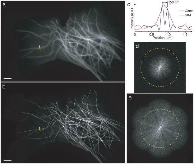
Comparison of conventional TIRF (a) and TIRF-SIM (b) images of the microtubule cytoskeleton in a single S2 cell. Scale bar 2 μm. (c) Normalized intensity profiles along the yellow lines in (a) (red curve) and (b) (blue curve). Two microtubules separated by ~150 nm are well resolved in the SIM reconstruction, but not by conventional microscopy. (d–e) Fourier transforms of the images in (a) and (b) respectively. The classical diffraction limit of the objective lens is indicated by a dashed circle of radius 5.96 μm⁻¹. Sample information is visible as a bright “starburst” in the low-spatial-frequency central region of (d). That it does not reach the diffraction limit indicates that the effective resolution is lower than theory predicts, as is true for most high-NA objectives. The same sample information features can be recognized in (e), where they continue out to significantly higher spatial frequencies, well beyond the diffraction limit. Time series videos of (a,b) and (d,e) are available as Supplementary Videos 1 and 2 online.

Figure 2

Time series live TIRF-SIM of EGFP-α-tubulin in an S2 cell. (a) Subset of one time frame (number 95) from a 180-frame sequence. Each frame was acquired in 270 ms (i.e., a raw data exposure time of 30 ms), using the full 512 × 512 pixel field of view of the camera. Time frames were deliberately spaced at 1 second intervals. (b) The green-boxed area of (a) shown at selected times as indicated, using conventional TIRF (left) or TIRF-SIM (right). The contrast of the conventional images has been increased for clarity. Green arrows indicate the end of one particular microtubule, which can be seen elongating until approximately the 100 s time point, and then rapidly shrinking; these changes are much easier to follow in the SIM reconstruction. (c) Maximum-intensity kymographs, using TIRF-SIM (top) and conventional TIRF (bottom), of the red-boxed area of (a). Five separate microtubules are seen expanding and contracting through the area. One microtubule in particular is retracting noticeably, causing tilted lines in the kymograph (blue arrow). Sharp transitions separate periods of steady polymerization or depolymerization from periods of constant length (examples indicated by yellow and orange brackets), or of slower and less stable growth or shrinkage (red bracket). Some constant-length periods are followed by resumed polymerization (orange bracket), others by rapid depolymerization (yellow bracket). Scale bars, 2 μm. A time series video and a three-dimensional kymograph of this data set are available as Supplementary Videos 5 and 6 online.

Figure 3

Time series live TIRF-SIM of kinesin-73-EGFP in an S2 cell. (a–b) Conventional TIRF (a) and TIRF-SIM (b) images of the first of 120 time frames. Each frame was acquired in 144 ms (i.e., a raw data exposure time of 16 ms), using a 256 × 256 pixel field of view. (c) Projection of the first 20 TIRF-SIM time frames, color-coded for time. Moving and stationary kinesin-cargo complexes can be seen as multi-colored curves and white spots respectively. (d) 3D maximum-intensity kymograph of the area red-boxed in (b), covering the first 80 time frames. Kinesin spots exhibited a variety of behaviors, including clustering together (red arrowhead), splitting or separating (yellow arrowhead), remaining stationary (vertical line between the green arrowheads), and traveling at a constant velocity (inclined straight line between the blue arrowheads). (e) Kymograph produced by maximum-intensity-projecting the area blue-boxed in (b), for the first 46 time points, onto the y-t plane. A traveling kinesin complex (red arrow) joined a nearly stationary kinesin complex (bottom center), and halted. After a 0.6 s pause, one kinesin complex traveled onward (yellow arrow), while the other remained stationary for another 1.8 s, at which time it also resumed forward travel (green arrow). A third kinesin complex that traveled past later, possibly along the same microtubule, did not pause (blue arrow). Scale bars, 2 μm (a–c) and 0.5 μm (e). Videos of this data set are available as Supplementary Videos 7 and 8 online.