Extracting kinematic parameters for monkey bipedal walking from cortical neuronal ensemble activity

Abstract

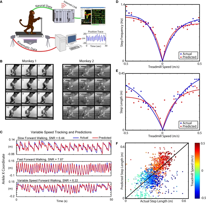
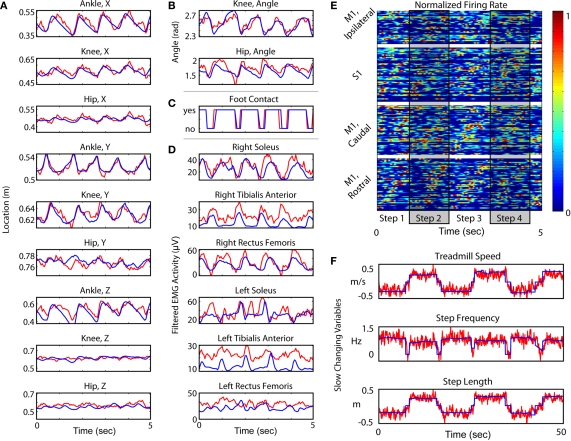
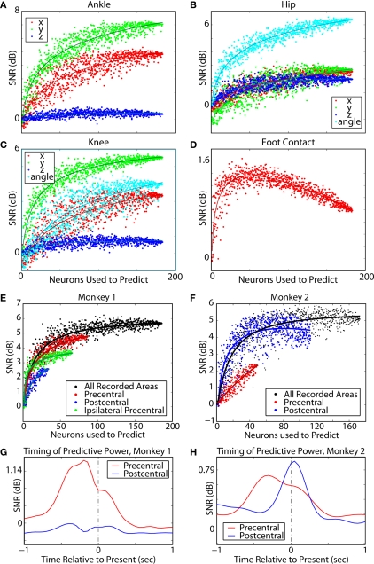
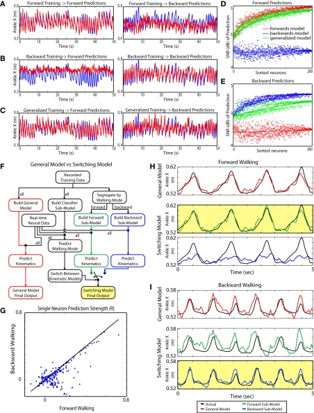
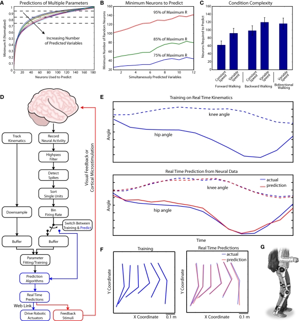
The ability to walk may be critically impacted as the result of neurological injury or disease. While recent advances in brain-machine interfaces (BMIs) have demonstrated the feasibility of upper-limb neuroprostheses, BMIs have not been evaluated as a means to restore walking. Here, we demonstrate that chronic recordings from ensembles of cortical neurons can be used to predict the kinematics of bipedal walking in rhesus macaques - both offline and in real time. Linear decoders extracted 3D coordinates of leg joints and leg muscle electromyograms from the activity of hundreds of cortical neurons. As more complex patterns of walking were produced by varying the gait speed and direction, larger neuronal populations were needed to accurately extract walking patterns. Extraction was further improved using a switching decoder which designated a submodel for each walking paradigm. We propose that BMIs may one day allow severely paralyzed patients to walk again.

Keywords: brain–machine interface; locomotion; neuronal ensemble recordings; neuroprosthetics; primate; sensorimotor.

Figure 1

Experimental setup and Kinematic Analysis. (A) Diagram of the bipedal walking setup, consisting of a custom modified, hydraulically driven treadmill; wireless, 2-camera tracking of kinematics; and a MAP neural acquisition system (Plexon, Inc., TX, USA). (B) Video frames traced from typical step cycles from both monkeys. (C) Example tracking at multiple speeds. (D) The relationship between step frequency and walking speed. Blue points and curves represent the actual values, and red points and curves represent the extracted values. Each point in (D) and (E) represents an average over an epoch of constant treadmill speed during variable speed and direction sessions. (E) The relationship between step length and walking speed. As in (C), blue and red correspond to the actual and predicted values, respectively. (F) Actual step lengths versus extracted step lengths during all variable speed sessions. Blue dots represent backward walking while red/orange dots represent forward (see key on the right). Dots are clustered around the y = x line, indicating a match between the actual and predicted values.

Figure 2

Diagram of cortical implants. A generic outline of cortical sulci (view from the top) is shown to illustrate the locations of the implants. Positive X coordinates correspond to rostral brain areas, while negative X coordinates correspond to caudal brain areas. (A) Implanted locations in Monkey 1. Both hemispheres were implanted. Two 32-electrode arrays were implanted in the left M1, one 32-electrode array in the left S1 and one 64-electrode array in the right M1. (B) Implanted locations in Monkey 2. The left hemisphere was implanted with two 64-electrode arrays, one placed in M1 and one in S1. (C–F) Configuration of the microelectrode arrays. The electrode shafts were arranged into 1-mm spaced grids. In multi-layered configurations, each shaft consisted of two (C,E) or four (D) microwires of different length. The difference in depth between the electrode layers was 0.3 mm.

Figure 3

Average changes in walking parameters during the step cycle. The data from all experimental sessions during which the monkey walked in forward direction with EMGs recorded were averaged. The average portions of the stance and swing phases of the step cycle are shown below each plot. The hip movements are not illustrated because they were small. Solid lines show the actual values, and dashed lines show the values extracted from neuronal activity using the Wiener filter. Note the correspondence between the actual and extracted values. (A–C) X, Y, and Z position. (D) Knee angle. (E) EMG activity in the muscles of the right leg. (F) Examples of leg orientations classified as swing and stance.

Figure 4

Neural activity in each cortical area during the step cycle. The neural data from experimental sessions during which the monkey walked in the forward and backward direction were separately averaged for many step cycles. Each horizontal line corresponds to the firing rate of a single neuron normalized by standard deviation (i.e. z-score). Each cortical area was analyzed separately (left M1 – top row, right M1 – middle row, left S1 – bottom row). The neurons were sorted by the phase of the step cycle during which they exhibited peak activity. The average durations of the stance and swing phases of the step cycle are shown below each plot. Swing was slightly longer during backwards walking. (A) Average neural activity during forward walking, ordered via peak activity during forward walking. (B) Average neural activity during backward walking, ordered via peak activity during backward walking. (C) Average neural activity during backward walking, ordered via peak activity during forward walking [i.e. neurons are ordered the same way in (A) and (C)].

Figure 5

Extraction of multiple characteristics of walking. In all traces, blue shows actual and red shows extracted value. All variables are shown over the same 5 s window, except in (F), where slow changing variables are shown over a longer 50 s window. (A) Three dimensional position variables. The X axis is in the direction of motion of the treadmill; the Y axis is off the surface of the treadmill (axis of gravity); and the Z axis is lateral to the surface of the treadmill, but orthogonal to the direction of motion. (B) Joint angle variables. Hip angle is calculated assuming a fixed torso. (C) Foot contact, a binary variable defining the swing versus stance phase. (D) EMG variables. (E) Neuronal activity of 220 single units sorted via cortical area and by phase within the step cycle. Firing rate is normalized for every unit. (F) Slow changing state variables (walking speed, step frequency and step length) plotted over a 50 s time window.

Figure 6

Neuronal dropping curves for simultaneously extracted variables. Dots represent SNR for the extraction of walking parameters using models trained on randomly selected neuronal populations of different sizes. In (A–C) red dots correspond to X coordinate, green dots to Y, and blue dots to Z. In (B,C) cyan dots correspond to joint angles for the respective joint. This analysis showed that prediction accuracy increased with the neuronal sample size [but see (D)]. Extraction analysis by cortical area was also performed for Monkey 1 (E,G) and Monkey 2 (F,H). In Monkey 1, more cells were recorded in M1 than in S1, whereas in Monkey 2 more cells were recorded in S1. (A) 3D coordinates of the ankle. (B) Joint angle and 3D coordinates of the knee. (C) Joint angle and 3D coordinates of the hip. (D) Foot contact, that is whether or not the monkey's foot was on the ground. Foot contact was well predicted for smaller numbers of neurons but experienced overfitting for large numbers of neurons. (E,F) Neuronal dropping curves for the entire neuronal population and separate areas with extrapolated fits. (G,H) Prediction accuracy for M1 (red curves) and S1 (blue curves) as a function of time lag between the time of prediction and the time at which neuronal activity was sampled. In Monkeys 1 and 2, precentral neurons best predicted current kinematics using neuronal data in the past, indicating that neuronal modulations preceded motion. Monkey 2's postcentral neurons had a peak in predictive power using future data, indicating that activity was a replica of the kinematics. In Monkey 1, the postcentral subpopulation did not have particularly strong predictive power in this analysis.

Figure 7

Generalized Training and the switching model. Panels A–C each represent a separate predictive model. In each, the left panel shows each model's ability to predict the kinematics of walking during sessions where the monkeys walk forward while the right panel shows each model's predictions of limb kinematics during periods of backward walking. The models accurately predicted conditions the same as the data they were trained upon but did not generalize well to conditions not contained within the training data set. The generalized model predicted either walking paradigm, but less accurately compared to paradigm-specific models. In response to these effects, a switching model (F–I) was designed that increased prediction accuracy for many kinematic parameters. (A) Actual and extracted traces of the X coordinate of the ankle for the forward walking model. Blue curves represent the actual position, and red curves represent the extracted position. (B) Traces for backward walking model. (C) Traces for generalized model. (D) Neuron dropping curves calculated by predicting forward walking using randomly selected neuronal populations with each model. (E) Neuron dropping curves calculated by predicting backward walking using randomly selected neuronal populations with each model. (F) Block diagram comparing the “switching” model with a generalized training model. Instead of using the same neuronal weights for all walking paradigms, the switching model uses two separate kinematic submodels running in parallel. Each model is optimized for a separate walking paradigm: forward and backward walking. A state predictive model determines walking mode and selects which of the two kinematic submodels becomes the final output. (G) Comparison of prediction strength of individual neurons during forward (abscissa) versus backwards (ordinate) walking. The prediction strength (R) was determined for single-neuron predictions of the X position of the ankle. While there is a general correlation between the Rs for these walking paradigms, there is a clear subpopulation of neurons with high Rs for forward, but not for backward walking. (H) Representative records of the X position of the ankle illustrating the predictive power of the switching model (the panel highlighted in yellow) versus generalized model (red curve) during forward walking. Note that the specialized model selected by the state predictive model (green curve) matches the original record (black curve) better than the generalized model (red curve) and the submodel for backward walking (blue curve). (I) Representative records for backward walking. The backward paradigm submodel selected by the state predictor (blue curve in the panel highlighted in yellow) matches the actual position (black curves) better than the generalized model (red curve) and the submodel for forward walking (green curve).

Figure 8

Simultaneous extraction of multiple parameters and real-time parameter extraction. (A) Neuronal dropping curves for extracting multiple parameters of walking. Each point on the curve represents the number of neurons needed to achieve a certain minimum level of prediction accuracy for each parameter (expressed as R normalized by the maximum value). The curves were fitted to the data for random groups of neurons used to predict random combinations of variables. This analysis revealed a slower rise for the multiple parameter dropping curves, indicating that larger neuronal populations were needed to predict multiple parameters simultaneously. (B) Number of neurons needed to attain a certain level of prediction accuracy (75%, 85% and 95% of maximum R) as the function of the number of simultaneously predicted variables. The curves were calculated from the neuron dropping curves shown in (A) These graphs show that the number of neurons needed for accurate prediction increased with the number of simultaneously extracted parameters of walking. (C) A comparison of the necessary number of neurons needed to accurately predict parameters in a variety of walking modes of different complexity. 95% of maximum R was set as the accuracy requirement. Bars show standard error. (D) Diagram outlining the operation of the real-time BMI. Real-time recordings of kinematic parameters and neural activity are filtered, binned and combined to train a series of Wiener models. Once the training is complete, the binned neural activity is sent into the models and kinematic output is generated. This kinematic output is used to drive robotic actuators. Feedback is sent back to the monkey using a visual display, or potentially, microstimulation pulses. (E) Training and prediction stages of the BMI. The panels show the average angles of hip and knee. In the top panel, training was occurring and there was not yet any predicted output. In the bottom panel extracted data was calculated (red), which matched actual kinematics (blue). (F) Training (left) and extraction (right) periods shown as the snapshots of leg configuration in treadmill surface centered coordinates. The configurations are projected onto the X–Y plane at 33 ms time steps to show a single step. Actual configurations of the leg are shown in blue, and predictions are shown in red. (G) Schematics of a future walking assist, exoskeletal BMI.

References

1. Alexander R. M. (2004). Bipedal animals, and their differences from humans. J. Anat. 204, 321–330. 10.1111/j.0021-8782.2004.00289.x - DOI - PMC - PubMed
1. Alkadhi H., Brugger P., Boendermaker S. H., Crelier G., Curt A., Hepp-Reymond M. C., Kollias S. S. (2005). What disconnection tells about motor imagery: evidence from paraplegic patients. Cereb. Cortex 15, 131–140. 10.1093/cercor/bhh116 - DOI - PubMed
1. Andriacchi T. P., Alexander E. J. (2000). Studies of human locomotion: past, present and future. J. Biomech. 33, 1217–1224. 10.1016/S0021-9290(00)00061-0 - DOI - PubMed
1. Armstrong D. M., Marple-Horvat D. E. (1996). Role of the cerebellum and motor cortex in the regulation of visually controlled locomotion. Can. J. Physiol. Pharmacol. 74, 443–455. 10.1139/cjpp-74-4-443 - DOI - PubMed
1. Azevedo C., Espiau B., Amblard B., Assaiante C. (2007). Bipedal locomotion: toward unified concepts in robotics and neuroscience. Biol. Cybern. 96, 209–228. 10.1007/s00422-006-0118-0 - DOI - PubMed