Mapping all-atom models onto one-bead Coarse Grained Models: general properties and applications to a minimal polypeptide model

Abstract

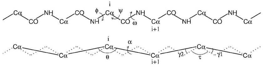
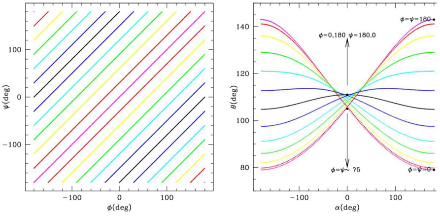
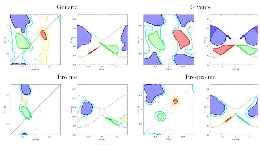
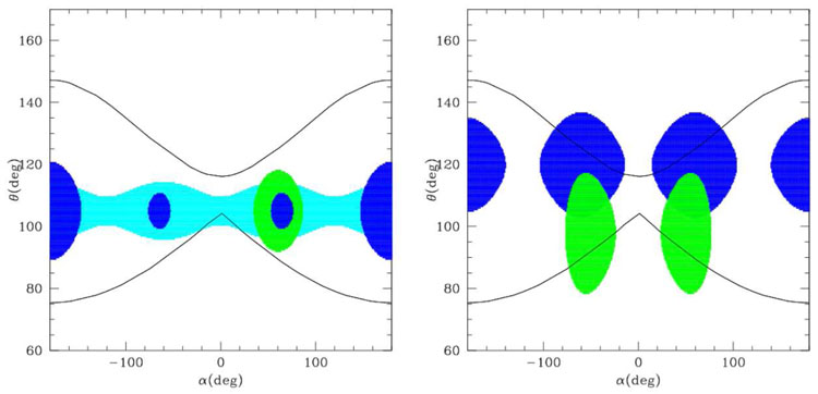
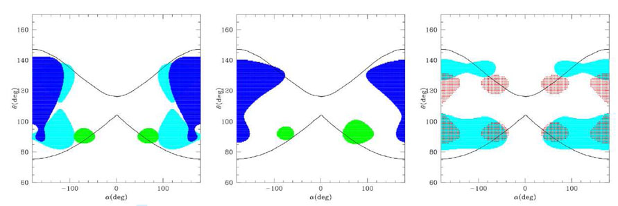
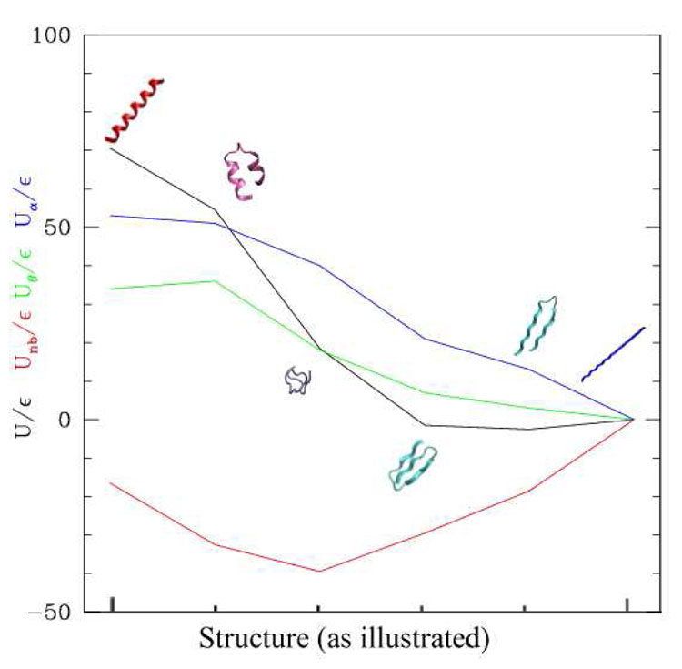
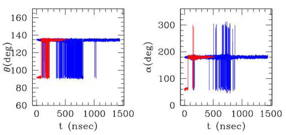
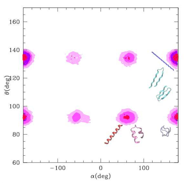
In the one and two beads Coarse Grained (CG) models for proteins, the two conformational dihedrals ϕ and ψ that describe the backbone geometry are no longer present as explicit internal coordinates, thus the information contained in the Ramachandran plot cannot be used directly. We derive an analytical mapping between these dihedrals and the internal variable describing the backbone conformation in the one(two) beads CG models, namely the pseudo-bond angle and pseudo-dihedral between subsequent Cαs. This is used to derive a new density plot that contains the same information as the Ramachandran plot and can be used with the one(two) beads CG models. The use of this mapping is then illustrated with a new one bead polypeptide model that accounts for transitions between α-helices and β-sheets.

Figure 1

Schematic representation of the coarse graining procedure. The internal coordinates (ϕ, ψ ω) and θ, α and the angles defining the CG geometry (τ, γ1; γ2) are reported.

Figure 2

Mapping of the ϕ, ψ plane onto the θ, α plane. Left: lines ϕ−ψ =cost are represented in different colors. Right: The same lines are mapped onto the α, θ plane. The region that they define is the image of the whole ϕ, ψ plane onto the α, θ plane through the (ϕ, ψ) → (α, θ) map. Some relevant points are reported.

Figure 3

Mapping of the Ramachandran plot onto the α, θ plane for different aminoacid types. The “core regions” are in green (right handed helices), red (left handed helices), blue (sheets). The allowed regions (yellow and cyan) are omitted in the Generic and Glycine α, θ plot for clarity. Forbidden regions are enclosed in the dotted lines. The contours of the “butterfly” image are reported as black lines in the α, θ plane. The input data for the Ramachandran plot are taken from the Protein Data Bank[18].

Figure 4

Typical α, θ density maps for two different kinds of FF. Left: Head-Gordon-like FF; right: Mukherjee-like FF. Green=helix, blue=sheet, cyan=turn.

Figure 5

α, θ density maps for the FF in the present work. Left: version with harmonic cosine dihedral potential; Center and right: version with cosine sum dihedral potential. Different maps are obtained giving different weights to the terms, in order to reproduce the map for sheet (blue), helix (green), glycine (cyan) and a generic model (red).

Figure 6

Relative stability and energy terms of the conformations explored during the simulations. Black: total potential energy, red = non bonded energy, green: bond angle energy, blue: dihedral energy. All energies are expressed in units of ∈. The extended conformation is taken as the zero-level. Parameters of the dihedral and bond angle terms: A = 2∈, B = 4∈, C = 0:5∈, D = 0, $\delta U_{\alpha }^{\theta }=7\in ,\delta U_{\alpha }^{\theta }=9\in$. Representative structures extracted from the simulations are reported: red=α-helix, pink=“broken-helix”, violet=random coil, cyan=β-hairpin and three-fold β-sheet.

Figure 7

“Representative values” of bond angles and dihedrals evaluated during the simulations starting from the α helix (red) and from the extended structure (blue). The “representative value” is evaluated as follows. For θ: for each timestep, all the 18 θ angles along the chain are measured, and two average values are calculated, one for the “extended” and one for the “helical” (conventionally separated by the value 113 deg). The representative value for θ is then chosen as the (average) value of the the most populated structure, for each timestep. For α: same procedure, except that in this case three separate average values are calculated for right handed (between 0 and 115 deg) or left handed helices (between −115 and 0) and for extended (otherwhise).

Figure 8

α, θ plot evaluated along the trajectories of the two simulations. Violet: simulation starting from the extended conformation. Pink-magenta-red: simulation starting from the α helix at increasing density values. The representative structures of the populated regions are reported.