Evolution of resource cycling in ecosystems and individuals

Abstract

Background: Resource cycling is a defining process in the maintenance of the biosphere. Microbial communities, ranging from simple to highly diverse, play a crucial role in this process. Yet the evolutionary adaptation and speciation of micro-organisms have rarely been studied in the context of resource cycling. In this study, our basic questions are how does a community evolve its resource usage and how are resource cycles partitioned?

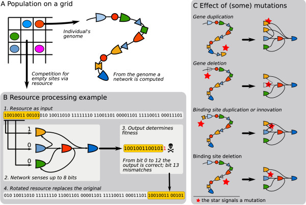
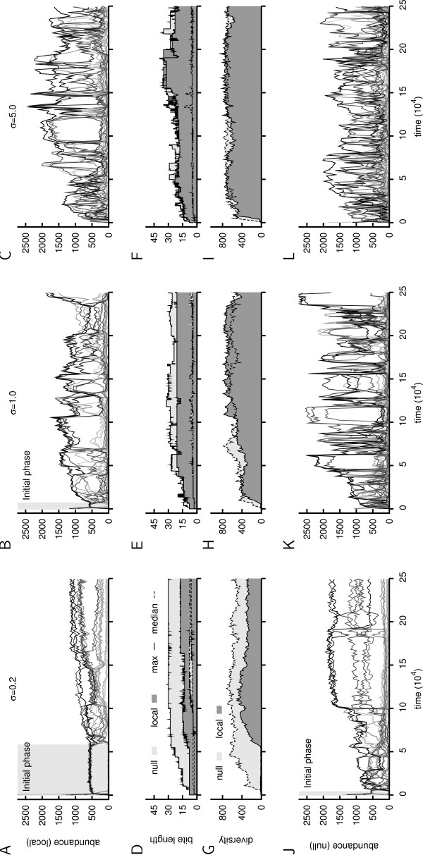
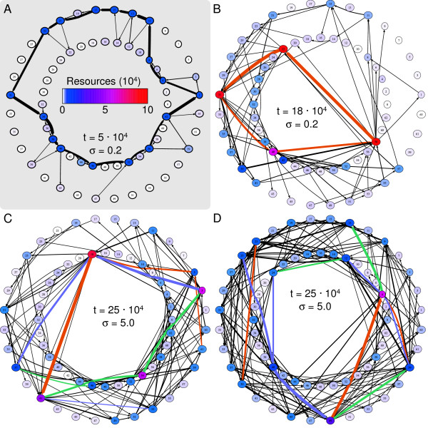
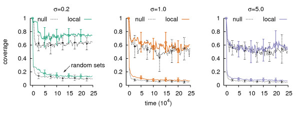
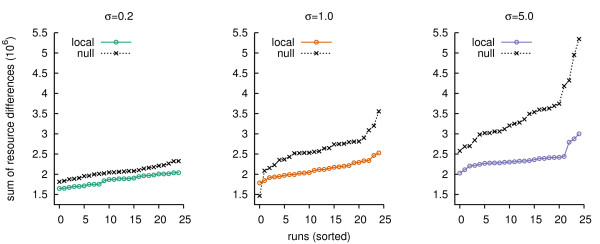
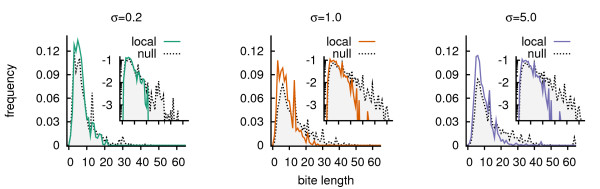
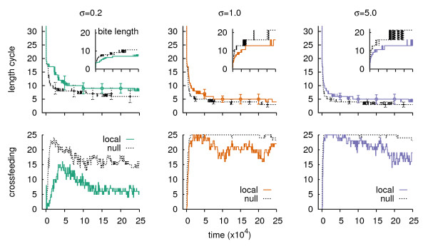
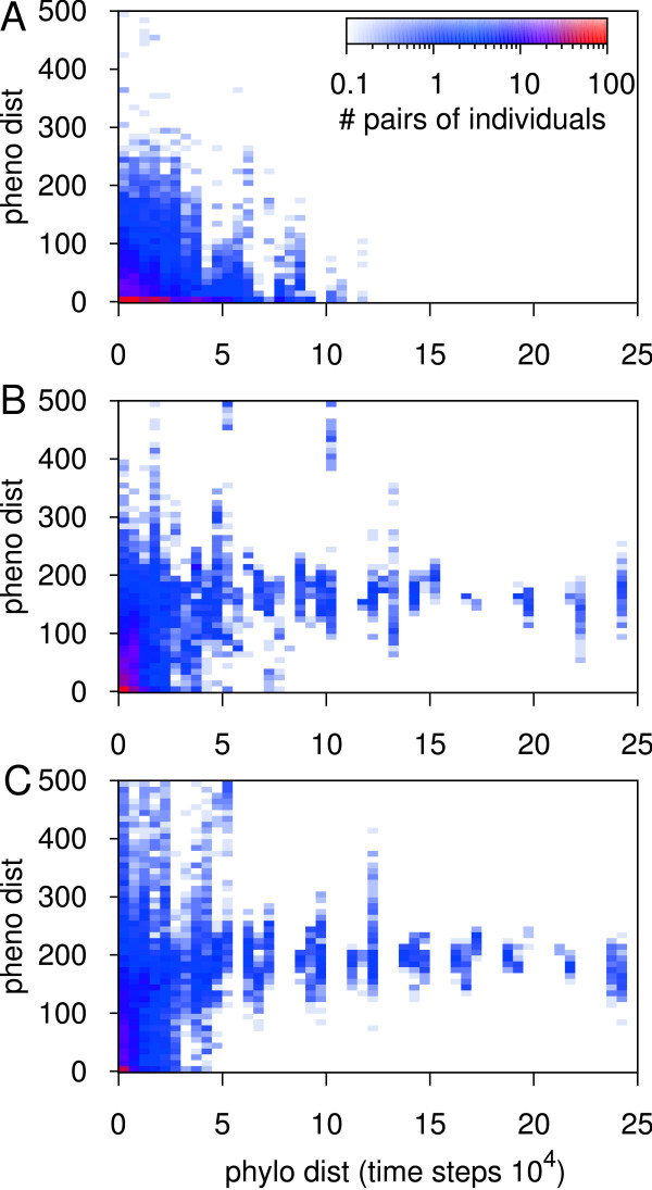
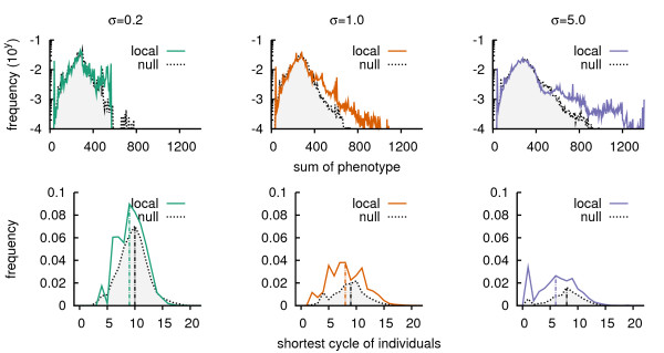
Results: We design a computational model in which a population of individuals evolves to take up nutrients and excrete waste. The waste of one individual is another's resource. Given a fixed amount of resources, this leads to resource cycles. We find that the shortest cycle dominates the ecological dynamics, and over evolutionary time its length is minimized. Initially a single lineage processes a long cycle of resources, later crossfeeding lineages arise. The evolutionary dynamics that follow are determined by the strength of indirect selection for resource cycling. We study indirect selection by changing the spatial setting and the strength of direct selection. If individuals are fixed at lattice sites or direct selection is low, indirect selection result in lineages that structure their local environment, leading to 'smart' individuals and stable patterns of resource dynamics. The individuals are good at cycling resources themselves and do this with a short cycle. On the other hand, if individuals randomly change position each time step, or direct selection is high, individuals are more prone to crossfeeding: an ecosystem based solution with turbulent resource dynamics, and individuals that are less capable of cycling resources themselves.

Conclusion: In a baseline model of ecosystem evolution we demonstrate different eco-evolutionary trajectories of resource cycling. By varying the strength of indirect selection through the spatial setting and direct selection, the integration of information by the evolutionary process leads to qualitatively different results from individual smartness to cooperative community structures.

Figure 1

Overview of the model. A. Individuals and resources are placed on a grid (size 100×100). Individuals consist of a genome, from which a network is computed. They compete for reproduction into empty grid sites by processing resources. B. The resource is a bit string of length 64. Maximally the first 8 bits can be sensed by a network, which then produces a sequence of bits at its output. The output is matched to the original bit string, and the length of the correct sequence (matching the bit string from the leftmost bit) is the raw score of the individual, which in this example is 13. If the individual reproduces, the resource is rotated from right to left for 13 bits and placed back in the grid site. C. The effect of a few types of mutation on the genome (left) and the topology of the network (right). By default the parameter values for each type of mutation are: gene duplication 16·10^-4, deletion 24·10^-4, binding specificity 4·10^-4, gene expression threshold 4·10^-4, binding site duplication 4·10^-4, deletion 10·10^-4, innovation 1·10^-4, binding specificity 4·10^-4, weight 4·10^-4. In order to balance the growth of the network, we apply a small penalty per gene and binding site of pen = 2.5·10^-5.

Figure 2

Resource abundance, population fitness and population diversity. A – C and J – L. The 20 most abundant resources are plotted through time. The darker a curve, the higher the abundance of this resource throughout the run. The top and bottom row contain, respectively, runs from the local and null model (for each selection regime a run). If visible at this scale, the initial phase is indicated by a gray background. D – F. Maximum and median fitness of the population through time. Dark shaded areas indicate the local model, light shaded areas the null model. G – I. Diversity in the population measured as the number of different network dynamics through time. Each 1000 time steps 1000 individuals were sampled and grouped by their network dynamics. The number of different groups is plotted. Grouping by phenotype gave qualitatively similar results.

Figure 3

Ecological views of several runs. Each 'wheel' shows the 64 resources (nodes) and the bites (edges) that rotate one resource into another. For visualization purposes even and odd numbered resources are plot on the inner and outer circle, respectively. Resources are colored by abundance, see the legend in panel A. The edge-width is logarithmically scaled according to popularity: the more a bite occurred the thicker the edge. In B, C and D the shortest cycles are colored to distinguish up to 3 different phenotypic groups (orange, purple and green). This coloring does not indicate any relationship between the phenotypes in different 'wheels'. A and C are taken from runs with local feedback (Figure 2A and C), B and D are from runs of the null model (Figure 2J and L). A. Run with low direct selection (σ = 0.2) at time 5·10⁴, which is still in the initial phase of evolution. B. Run with selection σ = 0.2 at time 18·10⁴. The shortest cycle (22, 31, 40, 58) is performed by a single lineage. C. Local model run with σ = 5.0 at time 25·10⁴. The shortest cycle (3, 18, 41, 54) is composed of three different phenotypic lineages. D. Null model run with σ = 5.0 at time 25·10⁴. There several shortest cycles, composed of multiple lineages. One of these cycles is: 4, 12, 24, 40, 49.

Figure 4

Resource coverage of shortest cycles. Mean coverage of the grid by resources on the shortest cycle, and random sets of resources. Coverage is expressed as a fraction of the total grid size. The random sets are composed of resources selected at random from the grid such that the size of the random set equals the number of resources on the shortest cycle.

Figure 5

Resource turbulence. For each run, we calculate for all resources the sum of absolute changes in resource abundance through time, and then sum over the resources. Thus we arrive at a single number indicating how turbulent resource dynamics have been through a run. For each selection regime the difference between the local and null model is statistically significant. For σ = 0.2, 1.0 and 5.0 the Wilcoxon rank-sum test (alternative hypothesis: local less than null) results in, respectively, p < 2.73·10^-6, p < 5.97·10^-8 and p < 1.38·10^-12.

Figure 6

Frequency distributions of bite lengths that lead to reproduction. The mean distributions are shown, summed over the period t = 12.5·10⁴ to 25·10⁴, and based on 25 runs of both the local and null model. The insets in the panels show the frequency plot in log scale, such that the differences in the tail are highlighted.

Figure 7

Shortest cycles, their length and crossfeeding. A. For the three selection regimes the mean shortest cycle with standard deviations is plotted through time. Inset panels show the corresponding average bite length on the shortest cycle. In all panels the mean and standard deviation are computed from 25 replicate runs. Using permutation tests, we established all three curves are significantly different (all p < 0.004). B. Number of runs with crossfeeding through time. In short, crossfeeding is present if the shortest cycle cannot be performed by a single group of phenotypically identical individuals, with the group having at least 5 individuals (see Methods).

Figure 8

Phylogenetic distance (phylo dist) against phenotypic distance (pheno dist). We computed phylogenetic trees of all runs with local feedback (for an example tree see additional file 2: Figure S1), and for each run we sampled a 1000 random pairs of individuals with a time of birth difference < 20 time steps and traced their last common ancestor. The phylogenetic distance is the difference in time of birth between the pair and their ancestor. Phenotypic distance is expressed as the Manhattan distance between two phenotypes. The colors, as given in the legend, give the number of pairs averaged over 25 runs. Note that the regular spacing in the data of B and C is an artifact of the periodicity of logging populations. Low, average and high selection are shown in A, B and C respectively (σ = 0.2, 1.0 and 5.0).

Figure 9

Distributions of individual 'smartness'. In both series of frequency plots we have taken per 1000 time steps a sample of 100 individuals, over the interval [12.5·10⁴, 25·10⁴]. With 6 × 25 runs this results in 6 data sets of 325000 individuals. A. Frequency plot of smartness defined as the sum of an individual's phenotype. Note the logarithmic y-axis. B. Frequency plot of smartness as an individual's shortest cycle. We calculated the shortest cycle given the presence of the most abundant resources at each sampling point. A minimal number of resources was selected such that the grid was covered by a 0.95 fraction. The three panels show the distribution of shortest cycle lengths of individuals that could actually perform a cycle. For individuals that were incapable of doing so see additional file 4: Figure S3.

References

-
- Treves DS, Manning S, J A. Repeated evolution of an acetate-crossfeeding polymorphism in long-term populations of Escherichia coli. Mol Biol Evol. 1998;15:789–797. - PubMed
- Porcher E, Tenaillon O, Godelle B. From metabolism to polymorphism in bacterial populations: a theoretical study. Evolution. 2001;55:2181–2193. - PubMed
Publication types
MeSH terms
LinkOut - more resources
Full Text Sources